import calendar
import matplotlib.pyplot as plt
import numpy as npWorking with numpy vectors
Introduction
This task requires working with numpy vectors and Python to conduct a data analysis exercise involving the price of Bitcoin in US dollars (BTC-USD) for 2023. The BTC-USD data is loaded into a numpy vector from a text file. Numpy vector operations are used to calculate some descriptive statistics for the third financial quarter. The Bitcoin price in US dollars is plotted using the Matplitlib library, with a function defined to allow any financial quarter or year to be plotted using the same lines of code. The daily Bitcoin price variation is investigated through a box plot and analysis of outliers.
Data input
The historical data for BTC-USD is available on the Yahoo finance website: https://finance.yahoo.com/quote/BTC-USD>. The data file contains the Bitcoin price data from 1st January 2023 to 8th March 2025 and is loaded using the loadtxt function from numpy.
rates = np.loadtxt("btc-usd_data.txt")Year for analysis
The loaded data starts on 1st January 2023 to 8th March 2025. We have data for the complete years 2023 and 2024. The variable below can be set to 2023 or 2024. The task requires data analysis of 2023, so the year variable is set to 2023.
year = 2023Helper function for handling different financial quarters and years in the data
The function get_year_info returns a dictionary containing information about the indices in the data for the start and end of the year and each of the financial quarters. This will be used to slice the data when doing the analysis below.
def get_year_info(chosen_year, data_start_year=2023):
    """
    For a given chosen_year, determines, the indexes for the chosen_year start and end, the start
    and end indices for each financial quarter and the number of days in the chosen_year.
    The function handles leap years.

    :param chosen_year: The year we need the information for.
    :param data_start_year: The year the data starts from. Defaulted to 2023.
    :return: A dictionary containing information for the indexes in the loaded data relating to the
        start and end of the various financial quarters.
    """
    # Initialise the result to an empty dictionary.
    result = {}

    # Ensure the input chosen_year is either 2023 or 2024
    if chosen_year not in [data_start_year, data_start_year + 1]:
        print(f"Year must be {data_start_year} or {data_start_year + 1}")
        return

    # Use the calendar module to check if the chosen_year is a leap year.
    if calendar.isleap(chosen_year):
        result["num_days_year"] = 366
        q1_num_days = 91
    else:
        result["num_days_year"] = 365
        q1_num_days = 90

    # Number of days in quarters 2,3 are independent on the chosen_year being a leap year.
    q2_num_days = 91
    q3_num_days = 92

    # Store the chosen_year's start and end indices
    result["year_start_num"] = 1
    result["year_end_num"] = result["num_days_year"]

    # For 2024 the data occurs after 2023 so update the start and end indices
    if chosen_year == data_start_year + 1:
        result["year_start_num"] = result["num_days_year"]
        result["year_end_num"] = result["year_start_num"] + result["num_days_year"] - 1

        # Add data into dictionary
    result["q1_start"] = result["year_start_num"]
    result["q1_end"] = result["q1_start"] + q1_num_days - 1
    result["q2_start"] = result["q1_end"] + 1
    result["q2_end"] = result["q2_start"] + q2_num_days - 1
    result["q3_start"] = result["q2_end"] + 1
    result["q3_end"] = result["q3_start"] + q3_num_days - 1
    result["q4_start"] = result["q3_end"] + 1
    result["q4_end"] = result["year_end_num"]

    return result
Get information about the year for analysis
Call get_year_info for the chosen year to obtain a dictionary that contains information relating to the indexes in the loaded data relating to the start and end of the various financial quarters.
year_info = get_year_info(year)Descriptive Statistics for Q3 for the chosen year
The following descriptive statistics are calculated using numpy functions and printed for Q3 of the chosen year:
- Arithmetic mean
- Minimum
- 1st quartile
- Median
- 3rd quartile
- Maximum
- Standard deviation
- Inter-quartile range (IQR)
The above calculations are done for the chosen financial quarter in the selected year, which, in this case, is Q3 2023. The quarter can be changed by changing the slicing used to create the numpy array fin_quarter, and the year can be changed with the variable year found at the top of the notebook.
# Create numpy array for the required quarter by slicing the full data
fin_quarter = rates[year_info["q3_start"]-1:year_info["q3_end"] ]

# Spacing to help with formatting of the printing
padding = 30

# Print the header
print(f"\033[1m  Descriptive Statistics for Q3 {year}\033[0m")

# Arithmetic mean
quarter_a_mean = np.mean(fin_quarter)
print(f"##{'arithmetic mean:':>{padding}}   {round(quarter_a_mean, 2):9.2f}")

# Minimum
quarter_min = np.min(fin_quarter)
print(f"##{'minimum:':>{padding}}   {round(quarter_min, 2):9.2f}")

# Quartiles, Q1, Median, Q3
quartiles = np.quantile(fin_quarter, [0, 0.25, 0.5, 0.75, 1])

# Q1 - first quartile
quarter_q1 = quartiles[1]
print(f"##{'Q1:':>{padding}}   {round(quarter_q1,2):9.2f}")

# Median
quarter_median = quartiles[2]
print(f"##{'median:':>{padding}}   {round(quarter_median, 2):9.2f}")

# Q3 - third quartile
quarter_q3 = quartiles[3]
print(f"##{'Q3:':>{padding}}   {round(quarter_q3, 2):9.2f}")

# Maximum
quarter_max = np.max(fin_quarter)
print(f"##{'maximum:':>{padding}}   {round(quarter_max, 2):9.2f}")

# Standard deviation
quarter_std = np.std(fin_quarter, ddof=0)
print(f"##{'standard deviation:':>{padding}}   {round(quarter_std, 3):9.2f}")

# Inter-quartile range (IQR)
quarter_iqr = quarter_q3 - quarter_q1
print(f"##{'IQR:':>{padding}}   {round(quarter_iqr, 3):9.2f}")
Descriptive Statistics for Q3 2023
## arithmetic mean: 28091.33
## minimum: 25162.65
## Q1: 26225.55
## median: 28871.82
## Q3: 29767.07
## maximum: 31476.05
## standard deviation: 1827.04
## IQR: 3541.51
During the 3rd financial quarter of 2023, the Bitcoin price had a minimum of \(\$25,162.25\) USD, a maximum of \(\$31,476.05\) USD and a standard deviation of \(\$1,827.04\) USD.
Plot of Bitcoin price value in USD for Q3 2023
Function for generating line plots of the data
The plot_quarter_year function takes the start, end and year start indices for slicing of the rates numpy array. Any financial quarter or year can be plotted by changing the slice start and end indices.
def plot_quarter_year(start, end, year_start, colour, label):
    """
    Generate a plot of the Bitcoin price as a function of days for either a financial quarter or
    calendar chosen_year.

    :param start: The index where the plotting will start in the complete data.
    :param end: The index in the complete data where the plotting will end.
    :param year_start: The index in the complete data for the start of the chosen chosen_year.
    :param colour: The colour for the line in the plot.
    :param label: The label to give the line in the plot.
    :return: A dictionary containing information for the indexes in the loaded data relating to the
        start and end of the various financial quarters.
    """
    # Create a numpy array that will be used for the x-axis in the plot
    days = np.arange(start - year_start + 1, end - year_start + 2)
    # Create the plot
    plt.plot(days, rates[start:end + 1], color=colour, label=label)
    plt.title("BTC to USD")
    plt.ylabel("Price of BTC in $US")
    plt.xlabel(f"Day number in {year}")
    plt.legend()
    plt.show()
Call the function to generate the plot
# Call the plot_quarter_year function using the Q3 start and end indices to choosing Q3 from rates
plot_quarter_year(year_info["q3_start"], year_info["q3_end"], year_info["year_start_num"], 'red',
                  f'Q3 {year}')
In the third quarter of 2023, the Bitcoin price started nearing its maximum value for the quarter. There was a gradual decline in price until days 228, then a sudden drop to ~\(\$26,000\) USD in a day. The price then gradually declined to the minimum for the quarter before rallying to finish the quarter at around \(\$28,000\) USD.
Highest and Lowest days
The numpy, armin, and argmax functions are used to calculate the index in the quarter’s numpy array where the minimum and maximum occur. This index is then adjusted to represent the day number in the year.
min_index = np.argmin(fin_quarter)
# Change the index to the day within the whole chosen_year rather than just the quarter
min_index += (year_info['q3_start'] - year_info["year_start_num"] + 1)
print(f"{'## Lowest':<10} price was on day {min_index} ({round(quarter_min, 2)}).")

max_index = np.argmax(fin_quarter)
# Change the index to the day within the whole chosen_year rather than just the quarter
max_index += (year_info['q3_start'] - year_info["year_start_num"] + 1)
print(f"## Highest price was on day {max_index} ({round(quarter_max, 2)}).")
## Lowest price was on day 254 (25162.65).
## Highest price was on day 194 (31476.05).For the third quarter of 2023, the highest price occurred on day 194 (July 13th) and the lowest on day 254 (September 11th).
Plots for Q1, Q2 and Q4 of 2023
# Call the plot_quarter_year function using the Q1 start and end indices to choosing Q1 from rates
plot_quarter_year(year_info["q1_start"], year_info["q1_end"], year_info["year_start_num"], 'green',
                  f'Q1 {year}')

# Call the plot_quarter_year function using the Q2 start and end indices to choosing Q3 from rates
plot_quarter_year(year_info["q2_start"], year_info["q2_end"], year_info["year_start_num"], 'orange',
                  f'Q2 {year}')

# Call the plot_quarter_year function using the Q3 start and end indices to choosing Q3 from rates
plot_quarter_year(year_info["q3_start"], year_info["q3_end"], year_info["year_start_num"], 'red',
                  f'Q3 {year}')

# Call the plot_quarter_year function using the Q4 start and end indices to choosing Q3 from rates
plot_quarter_year(year_info["q4_start"], year_info["q4_end"], year_info["year_start_num"], 'blue',
                  f'Q4 {year}')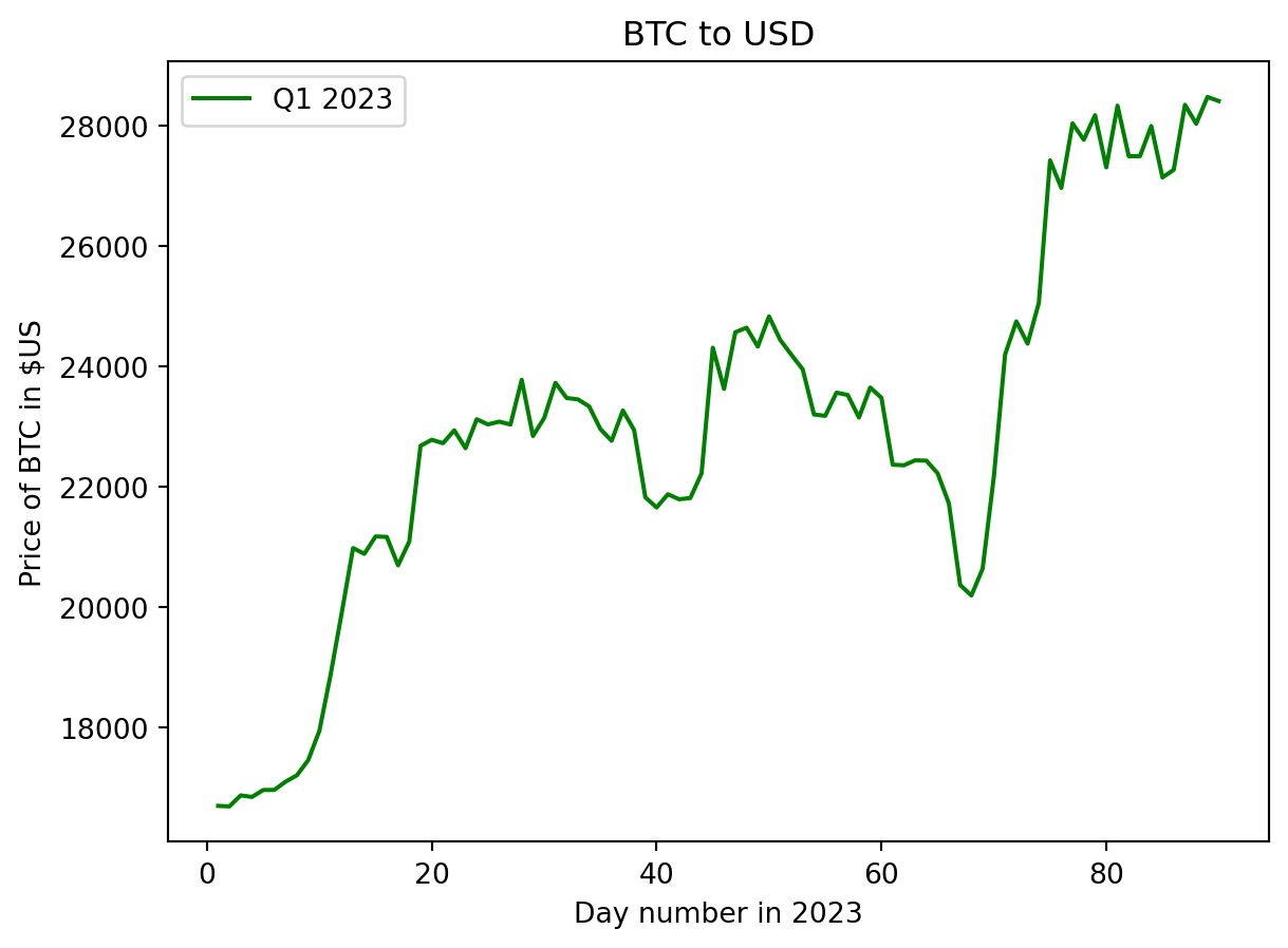
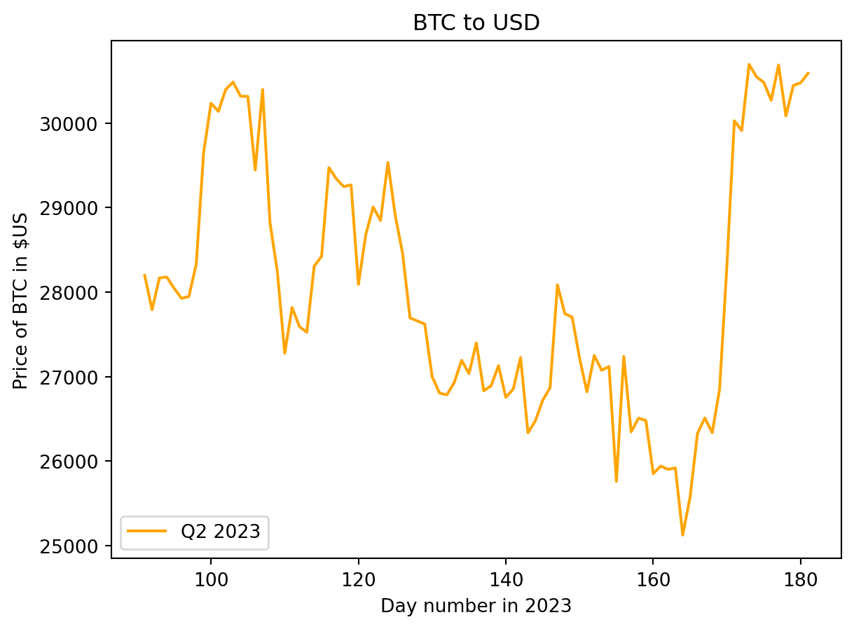
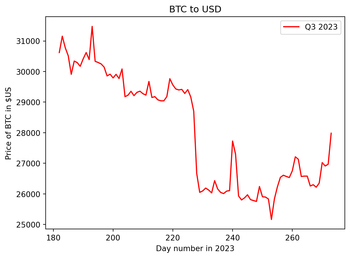
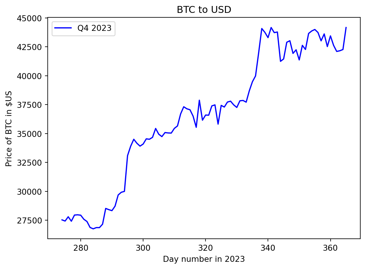
The Bitcoin price started 2023 around \(\$16,500\) USD and showed bullish behaviour to finish the quarter near \(\$28,000\) USD. Performance in the 2nd quarter shows high variability, with the overall trend decreasing to the lowest value of ~ \(\$25,000\) USD on June 15th before a dramatic rise to close the quarter around \(\$30,500\) USD. The bullish behaviour seen at the end of the 3rd quarter carried into the 4th quarter. A jump in price from \(\$30,000\) USD to ~ \(\$34,500\) USD occurred between days 296 and 300 (October 23rd to 26th), with another strong rally from \(\$37,800\) USD to \(\$44,000\) USD between days 335 and 340 ( December 1st to 6th). The price stabilises during December to finish the quart and year at \(\$42,152.10\) USD.
Box-and-whisker plot for price variation in Q3 in 2023
To understand the daily Bitcoin price variation, a box-and-whisker plot can be created from the daily increase/decrease in price.
The daily variation in price for a quarter can be calculated using numpy.diff.
quarter_price_difference = np.diff(fin_quarter)Create the plot
Use the Matplotlib boxplot function to create the plot. The figure size is adjusted to reduce the vertical white space in the plot and to increase its width. The arithmetic mean of the quarter daily price difference is calculated using numpy.mean and added to the plot with the Matplotlib plot function.
plt.figure(figsize=(12, 3), )
plt.boxplot(quarter_price_difference, vert=False)
plt.plot(np.mean(quarter_price_difference), 1, color='green', marker='x', linewidth=2, markersize=10)
plt.title(f"Distribution of BTC-to-USD daily price increases in Q3 {year}")
plt.yticks([], [])
plt.show()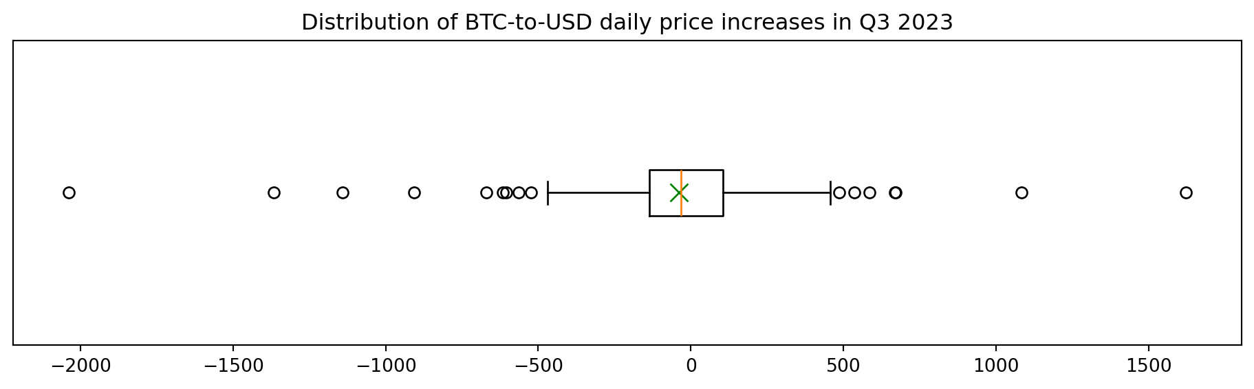
The box plot shows a graphical representation of some of the descriptive statistics. The left side of the box is the first quartile, the right side is the third quartile, and the orange line inside the box is the median. The box length is the difference between the third and first quartiles and represents the inter-quartile range (IQR) and represents 50% of the data. The whiskers are placed at 1.5*IQR above and below the third and first quartiles. Values outside the whiskers are termed outliers.
Counting outliers
Outliers are values that are outside the whiskers. Low outliers are below Q1-1.5IQR, and high outliers are above Q3+1.5IQR. The number of outliers can be counted by finding the values outside the whiskers using slicing. The number is simply the length of the resulting arrays.
# Count outliers
# Quartiles, Q1, Median, Q3
difference_quartiles = np.quantile(quarter_price_difference, [0.25, 0.75])

# Q1
quarter_difference_q1 = difference_quartiles[0]

# Q3
quarter_difference_q3 = difference_quartiles[1]

# Inter quartile range (IQR)
quarter_difference_iqr = quarter_difference_q3 - quarter_difference_q1

# Calculate the values for the whiskers
lower_whisker = quarter_difference_q1 - 1.5 * quarter_difference_iqr
upper_whisker = quarter_difference_q3 + 1.5 * quarter_difference_iqr

# Create arrays only containing values outside the whiskers
outliers_above = quarter_price_difference[quarter_price_difference > upper_whisker]
outliers_below = quarter_price_difference[quarter_price_difference < lower_whisker]

# The length of the arrays represents the number of outliers.
print(f"## There are {len(outliers_above) + len(outliers_below)} outliers.",
      f"{len(outliers_above)} above the right whisker and",
      f"{len(outliers_below)} below the left whisker.")
## There are 16 outliers. 7 above the right whisker and 9 below the left whisker.Bitcoin’s price can have extreme price fluctuations in short periods of time, and these are likely to appear as outliers.
Summary
This Jupyter Notebook demonstrates the use of numpy vectors and functions to analyze Bitcoin price data quantitatively using descriptive statistics and visually using line and box plots.
Possible extensions to the data analysis include: - Create a box plot for each financial quarter to visually compare the daily price difference between quarters. - Plot the price difference data as a histogram and compare to a normal model. - Extend the analysis to look at other years.