Drug Induced Autoimmunity

import os
import pandas as pd
import numpy as np

from sklearn.metrics import roc_auc_score, roc_curve, auc, accuracy_score, matthews_corrcoef, confusion_matrix
from sklearn.model_selection import cross_val_predict

import warnings
warnings.filterwarnings('ignore')

Introduction

This notebook is concerned with the results of the research paper InterDIA: Interpretable prediction of drug-induced autoimmunity through ensemble machine learning approaches by Lina Huang, Peineng Liu and Xiapjie Huang, published in Toxicology 2025. This work has two parts:

• Part 1: focuses on reproducing the main results (feature subset RDKit_GA_65) from the publication, presented in Table 5 on page 5.
• Part 2: focuses on the design and development of my own machine learning solution to this problem.

Load feature list

To get the features in the RDKit_GA_65 feature subset, the supplementary data associated with this article from doi:10.1016/j.tox.2025.154064 was used. The supplementary data is provided as an Excel file with the list of features for the subset available on the “Tabel S4” sheet.

# Load feature lists
# Excel file with supplementary information
file_path = "data/1-s2.0-S0300483X25000204-mmc1.xlsx"

# Load the specific sheet containing the feature lists
supp_df = pd.read_excel(file_path,  sheet_name="Table S4", index_col=None, header=2)

# Extract the RDKit_GA_65 column into a list
rdkit_ga_65 = supp_df.iloc[:, 1].dropna().tolist()

# Print or use the lists
print("RDKit_GA_65")
print(f"Number of descriptors: {len(rdkit_ga_65)}")

feature_sets = {"RDKit_GA_65": rdkit_ga_65,}

RDKit_GA_65
Number of descriptors: 65

Load data

The dataset used in this notebook is the Drug Induced Autoimmunity Prediction dataset from the UC Irvine Machine Learning Repository. The data is licensed under CC BY, allowing it to be freely used for this exercise. This dataset corresponds to the data used in the paper.

The data comprises 192 features, one labelled variable, “Label” and one categorical variable “SMILES”. The SMILES (Simplified Molecular Input Line Entry System) are a standardised text-based language for describing the structure of chemical molecules using short ASCII strings. For this work, “Label” is used as the target variable.

# Load datasets
train_df = pd.read_csv("data/DIA_trainingset_RDKit_descriptors.csv")  
test_df = pd.read_csv("data/DIA_testset_RDKit_descriptors.csv")

print(f"Training data shape: {train_df.shape}")
print(f"Testing data shape: {test_df.shape}")
 
# Count the number of 0s and 1s
train_counts = train_df["Label"].value_counts()
test_counts = test_df["Label"].value_counts()

# Calculate the ratio of 0s to 1s
train_positive_count = train_counts.get(1, 1)
test_positive_count = test_counts.get(1, 1)
    
train_negative_count = train_counts.get(0, 0)
test_negative_count = test_counts.get(0, 0)
    
train_ratio = train_counts.get(0, 0) / train_counts.get(1, 1)
test_ratio = test_counts.get(0, 0) / test_counts.get(1, 1)

print(f"Number of DIA-positive drugs in Training set: {train_positive_count}")
print(f"Number of DIA-negative drugs in Training set: {train_negative_count}")
print(f"Ratio of negative to positive in Training set: {train_ratio:.2f}")
    
print(f"Number of DIA-positive drugs in External validation set: {test_positive_count}")
print(f"Number of DIA-negative drugs in External validation set: {test_negative_count}")
print(f"Ratio of negative to positive in External validation set: {test_ratio:.2f}")
print()

Training data shape: (477, 198)
Testing data shape: (120, 198)
Number of DIA-positive drugs in Training set: 118
Number of DIA-negative drugs in Training set: 359
Ratio of negative to positive in Training set: 3.04
Number of DIA-positive drugs in External validation set: 30
Number of DIA-negative drugs in External validation set: 90
Ratio of negative to positive in External validation set: 3.00

Part 1: Reproduce paper results

from sklearn.preprocessing import StandardScaler  
from sklearn.ensemble import GradientBoostingClassifier  
from sklearn.tree import DecisionTreeClassifier
from sklearn.ensemble import AdaBoostClassifier
from imblearn.ensemble import BalancedRandomForestClassifier, EasyEnsembleClassifier, BalancedBaggingClassifier  
from xgboost import XGBClassifier  
from lightgbm import LGBMClassifier  
from sklearn.model_selection import KFold

Global parameters

RANDOM_STATE = 1 # Key piece of information for reproducibility

# Define models and metrics names
MODEL_NAMES = ["BRF", "EEC", "BBC+XGBoost", "BBC+GBDT", "BBC+LightGBM"]
METRIC_NAMES = ["AUC", "ACC(%)", "SEN(%)", "SPE(%)", "MCC"]
EVALUATION_NAMES = ["10-fold cv", "External set"]

Helper functions

def calculate_metrics(y_true, y_pred, y_proba):  
    """
    Calculate the performance metrics as per Huang et al. (2025)

    :param y_true: True values.
    :param y_pred:  Predicted values.
    :param y_proba:  Prediction probabilities.
    :return: Dictionary with calculated metrics
    """
    # Get true/false positive/negative values from confusion matrix
    tn, fp, fn, tp = confusion_matrix(y_true, y_pred).ravel()  

    # Calculate accuracy score
    acc = accuracy_score(y_true, y_pred)  

    # Calculate sensitivity/recall
    sen = tp / (tp + fn)  

    # Calculate specificity
    spe = tn / (tn + fp)  

    # Calculate the Matthews correlation coefficient
    mcc = matthews_corrcoef(y_true, y_pred)  

    # Calculate the area under the curve 
    auc = roc_auc_score(y_true, y_proba)
    
    metrics = {
        "AUC": auc,
        "ACC": acc,
        "SEN": sen,
        "SPE": spe,
        "MCC": mcc
    } 
    return metrics


def initialise_dict(data_dict):
    """
    Initialises dictionary with the required structure.

    :param data_dict: Dictionary to initialise.
    :return: None
    """
    for m in MODEL_NAMES:
        data_dict.setdefault(m, {})
        for evaluation in EVALUATION_NAMES:
            data_dict[m][evaluation] = [0]*5


def update_values(fs_name, orig, repro, var, updates_lst):
    """
    Function to update the dictionaries for the reproduced_values and 
    variation_values.

    :param fs_name: Name of the feature set.
    :param orig: Dictionary containing original values from the journal paper.
    :param repro: Dictionary of values generated in this notebook.
    :param var: Dictionary of differences between original and reproduced values.
    :param updates_lst: List containing tuples with the updated values
    :return: None
    """
    for eval_type, m, repro_values in updates_lst:
        orig_values = orig[fs_name][m][eval_type]
        repro[m][eval_type] = repro_values
        var_values = [round(a - b, 4) for a, b in zip(orig_values, repro_values)]
        var[m][eval_type] = var_values


def create_latex_tables(fs_name, orig, repro, var):
    """
    Function to combine results into a table for exporting to Latex for reporting.

    :param fs_name: Name of the feature set.
    :param orig: Dictionary containing original values from the journal paper.
    :param repro: Dictionary of values generated in this notebook.
    :param var: Dictionary of differences between original and reproduced values.
    :return: None
    """
    # Create a list of rows for the combined table
    rows = []
    for m in MODEL_NAMES:
        for eval_type in EVALUATION_NAMES:
            for i, metric in enumerate(METRIC_NAMES):
                row = {
                    "Model": m if i == 0 and eval_type == EVALUATION_NAMES[0] else "",
                    "Evaluation": eval_type if i == 0 else "",
                    "Metric": metric,
                    "Original": str(orig[m][eval_type][i]),
                    "Reproduced": str(repro[m][eval_type][i]),
                    "Variation": str(var[m][eval_type][i])
                }
                rows.append(row)
                
    # Create DataFrame
    df_combined = pd.DataFrame(rows)

    # Generate LaTeX code
    latex_code = df_combined.to_latex(index=False, escape=True)

    # Save to file to include in report
    with open(f"{fs_name}_model_metrics_combined_table.tex", "w") as f:
        f.write(latex_code)

    return df_combined

Model definitions and hyperparameters

The models used in the paper are discussed on page 3, and the tuned hyperparameters are provided in Table S5 of the supplementary material. It was discovered that not all the required hyperparameters needed to reproduce the work were reported in Table S5. Those missing were ‘scale_pos_weight’ (BBC+XGBoost) and the random state, which were required by the models. The first is a parameter relating to class imbalance and could be deduced from the relevant documentation. The random state, on the other hand, cannot be inferred and would require running the models with different values and evaluating the results until the correct random state is found. Fortunately, the authors provided a link in the paper to a GitHub repository where the random state used for the paper was found.

# Model definitions with hyperparameters from table S5 of the supplementary material, and some from
# the paper's authors' GitHub repository
# https://github.com/Huangxiaojie2024/InterDIA/blob/main/DIA_RDKit_Prediction.ipynb

rdkit_ga_65_models = {
    "BRF": 
        BalancedRandomForestClassifier( # page 3
            n_estimators=154, # Table S5
            criterion="gini", # Table S5
            max_depth=15, # Table S5
            max_features=48, # Table S5
            random_state=RANDOM_STATE, # GitHub
            sampling_strategy="auto", # default - added to silence future warnings
            replacement=False, # default - added to silence future warnings
            bootstrap=True, # default - added to silence future warnings
        ),  
    "EEC":
        EasyEnsembleClassifier( # page 3
            estimator=AdaBoostClassifier( # page 3
                estimator=DecisionTreeClassifier(
                    max_depth=7, # Table S5
                    random_state=RANDOM_STATE # GitHub
                ),
                n_estimators=178, # Table S5
                learning_rate=0.92, # Table S5
                algorithm='SAMME.R', # Table S5
                random_state=RANDOM_STATE # GitHub
            ),
            random_state=RANDOM_STATE, # GitHub
        ),  
    "BBC+XGBoost":
        BalancedBaggingClassifier( # page 3 
            estimator=XGBClassifier(
                n_estimators=172, # Table S5
                learning_rate=0.73, # Table S5
                booster="dart", # Table S5
                colsample_bytree=0.3, # Table S5
                colsample_bynode=1.0, # Table S5
                gamma=0.036296772856035525, # Table S5
                reg_lambda=0.06781903189364931, # Table S5
                min_child_weight=1.0, # Table S5
                max_depth=18, # Table S5
                subsample=0.9, # Table S5
                scale_pos_weight=train_ratio, # GitHub
                random_state=RANDOM_STATE, # GitHub
            ),  
            random_state=RANDOM_STATE, # GitHub
        ),  
    "BBC+GBDT":
        BalancedBaggingClassifier(  
            estimator=GradientBoostingClassifier(
                n_estimators=107, # Table S5
                learning_rate=0.24, # Table S5
                criterion='friedman_mse', # Table S5
                max_depth=5, # Table S5
                max_features=4, # Table S5
                subsample=0.99, # Table S5
                random_state=RANDOM_STATE, # GitHub
            ),  
            random_state=RANDOM_STATE, # GitHub
        ),  
    "BBC+LightGBM":
        BalancedBaggingClassifier(  
            estimator=LGBMClassifier(
                boosting_type='gbdt', # Table S5
                n_estimators=112, # Table S5
                learning_rate=0.83, # Table S5
                max_depth=14, # Table S5
                num_leaves=85, # Table S5
                colsample_bytree=0.55, # Table S5
                subsample=0.83, # Table S5
                reg_alpha=0.011600450241817575, # Table S5
                reg_lambda=0.12670847895140583, # Table S5
                min_child_samples=2, # Table S5
                random_state=RANDOM_STATE, # GitHub
            ),  
            random_state=RANDOM_STATE, # GitHub
        )  
}

models = {
    "RDKit_GA_65" : rdkit_ga_65_models,
}

Results from the journal paper

The results for the RDKit_GA_65 feature set in Table 5 have been added into a dictionary for look-up later.

# Define the original values for each model and evaluation method
# These are the results presented in Table 5 of the journal paper.
original_values = {
    "RDKit_GA_65":
    {
        "BRF": {
            "10-fold cv": [0.8764, 81.76, 83.05, 81.34, 0.5841],
            "External set": [0.8878, 80.83, 76.67, 82.22, 0.5444]
        },
        "EEC": {
            "10-fold cv": [0.8836, 82.81, 82.20, 83.01, 0.5978],
            "External set": [0.8930, 85.00, 83.33, 85.56, 0.6413]
        },
        "BBC+XGBoost": {
            "10-fold cv": [0.8499, 79.87, 77.97, 80.50, 0.5327],
            "External set": [0.8763, 80.83, 73.33, 83.33, 0.5313]
        },
        "BBC+GBDT": {
            "10-fold cv": [0.8773, 83.65, 74.58, 86.63, 0.5850],
            "External set": [0.8974, 85.00, 73.33, 88.89, 0.6093]
        },
        "BBC+LightGBM": {
            "10-fold cv": [0.8653, 82.81, 74.58, 85.52, 0.5694],
            "External set": [0.8915, 84.17, 73.33, 87.78, 0.5926]
        }
    },
}
# Initialise dictionaries for the reproduced and variation results
reproduced_values = {}
variation_values = {}
initialise_dict(reproduced_values)
initialise_dict(variation_values)
compare_dfs = {}

Train and evaluate models

This section has been written assuming that more than one feature set may be used. So it starts by looping through all the provided feature sets. For each feature set, the list of features is used to filter the training and test data sets. A standard scaler is applied to the filtered data. A loop is used to process each model separately. The model is fit to the training data, and the performance metrics are evaluated and stored. At the same time, the false true positive and true positive rates are calculated and stored for comparison in part 2. After all the models have been built and evaluated, the last step is to combine all the data into a DataFrame and create a LaTeX version for the report. Printing of the combined results shows that only the AUC for the BRF model on the external training set varies from the published values. A comparison of this value from the paper, 0.8878, with that calculated here, 0.8887, suggests that potentially this is a recording error in the paper, with the last two digits being swapped.

roc_data = {}

for fset_name, feature_list in feature_sets.items():
    print(f"Reproducing results for Feature Subset: {fset_name}")
    
    # Prepare data for the current feature set
    X_train = train_df[feature_list]  
    y_train = train_df['Label']  
    X_test = test_df[feature_list]  
    y_test = test_df['Label']

    roc_data[fset_name] = {}
    
    # Preprocessing: Z-score normalisation, page 3.
    scaler = StandardScaler()  
    X_train_scaled = scaler.fit_transform(X_train)  
    X_test_scaled = scaler.transform(X_test)

    for model_name, model in models[fset_name].items():
        print(f"  Processing model: {model_name}")
        # 10-fold Cross-Validation on training set
        # Paper doesn't mention stratifying the cross-validation, so I won't stratify
        cv = KFold(n_splits=10, shuffle=True, random_state=RANDOM_STATE)
          
        # Get out-of-fold predictions and probabilities for the minority class
        y_pred_cv = cross_val_predict(model, X_train_scaled, y_train, cv=cv, n_jobs=-1)  
        y_proba_cv = cross_val_predict(model, X_train_scaled, y_train, cv=cv,
                                       method="predict_proba", n_jobs=-1)[:, 1]  

        # Calculate the evaluation metrics for the cross-validation results
        cv_metrics = calculate_metrics(y_train, y_pred_cv, y_proba_cv)

        # External Validation 
        # Train on the full training set
        model.fit(X_train_scaled, y_train)  
          
        # Predict on the external validation set  
        y_pred_ext = model.predict(X_test_scaled)  
        y_proba_ext = model.predict_proba(X_test_scaled)[:, 1]  

        # Calculate the evaluation metrics for the external validation set
        ext_metrics = calculate_metrics(y_test, y_pred_ext, y_proba_ext)  
        
        # Compute FPR, TPR, and thresholds
        fpr, tpr, _ = roc_curve(y_test, y_proba_ext)
        roc_auc = auc(fpr, tpr)

        # Store for plotting later
        roc_data[fset_name][model_name] = {'fpr': fpr, 'tpr': tpr, 'auc': roc_auc}

        # Create a list of values for insertion into the dictionary
        cv_values_list = [
            round(cv_metrics['AUC'], 4),
            round(cv_metrics['ACC'] * 100, 2),
            round(cv_metrics['SEN'] * 100, 2),
            round(cv_metrics['SPE'] * 100, 2),
            round(cv_metrics['MCC'], 4)
        ]

        # Create a list of values for insertion into the dictionary
        ext_values_list = [
            round(ext_metrics['AUC'], 4),
            round(ext_metrics['ACC'] * 100, 2),
            round(ext_metrics['SEN'] * 100, 2),
            round(ext_metrics['SPE'] * 100, 2),
            round(ext_metrics['MCC'], 4)
        ]

        # Create updates list for this model
        updates = [
            ("10-fold cv", model_name, cv_values_list),
            ("External set", model_name, ext_values_list)
        ]

        # Update the values in the dictionary for this model
        update_values(fset_name, original_values, reproduced_values, variation_values, updates)

    # Create a combined DataFrame with all results, presented the same as the report.
    combined_df = create_latex_tables(fset_name, original_values[fset_name], reproduced_values, variation_values)
    compare_dfs[fset_name] = combined_df 

Reproducing results for Feature Subset: RDKit_GA_65
  Processing model: BRF
  Processing model: EEC
  Processing model: BBC+XGBoost
  Processing model: BBC+GBDT
  Processing model: BBC+LightGBM

# Show the combined results
print(compare_dfs["RDKit_GA_65"].to_string(index=False))

       Model   Evaluation Metric Original Reproduced Variation
         BRF   10-fold cv    AUC   0.8764     0.8764       0.0
                          ACC(%)    81.76      81.76       0.0
                          SEN(%)    83.05      83.05       0.0
                          SPE(%)    81.34      81.34       0.0
                             MCC   0.5841     0.5841       0.0
             External set    AUC   0.8878     0.8887   -0.0009
                          ACC(%)    80.83      80.83       0.0
                          SEN(%)    76.67      76.67       0.0
                          SPE(%)    82.22      82.22       0.0
                             MCC   0.5444     0.5444       0.0
         EEC   10-fold cv    AUC   0.8836     0.8836       0.0
                          ACC(%)    82.81      82.81       0.0
                          SEN(%)     82.2       82.2       0.0
                          SPE(%)    83.01      83.01       0.0
                             MCC   0.5978     0.5978       0.0
             External set    AUC    0.893      0.893       0.0
                          ACC(%)     85.0       85.0       0.0
                          SEN(%)    83.33      83.33       0.0
                          SPE(%)    85.56      85.56       0.0
                             MCC   0.6413     0.6413       0.0
 BBC+XGBoost   10-fold cv    AUC   0.8499     0.8499       0.0
                          ACC(%)    79.87      79.87       0.0
                          SEN(%)    77.97      77.97       0.0
                          SPE(%)     80.5       80.5       0.0
                             MCC   0.5327     0.5327       0.0
             External set    AUC   0.8763     0.8763       0.0
                          ACC(%)    80.83      80.83       0.0
                          SEN(%)    73.33      73.33       0.0
                          SPE(%)    83.33      83.33       0.0
                             MCC   0.5313     0.5313       0.0
    BBC+GBDT   10-fold cv    AUC   0.8773     0.8773       0.0
                          ACC(%)    83.65      83.65       0.0
                          SEN(%)    74.58      74.58       0.0
                          SPE(%)    86.63      86.63       0.0
                             MCC    0.585      0.585       0.0
             External set    AUC   0.8974     0.8974       0.0
                          ACC(%)     85.0       85.0       0.0
                          SEN(%)    73.33      73.33       0.0
                          SPE(%)    88.89      88.89       0.0
                             MCC   0.6093     0.6093       0.0
BBC+LightGBM   10-fold cv    AUC   0.8653     0.8653       0.0
                          ACC(%)    82.81      82.81       0.0
                          SEN(%)    74.58      74.58       0.0
                          SPE(%)    85.52      85.52       0.0
                             MCC   0.5694     0.5694       0.0
             External set    AUC   0.8915     0.8915       0.0
                          ACC(%)    84.17      84.17       0.0
                          SEN(%)    73.33      73.33       0.0
                          SPE(%)    87.78      87.78       0.0
                             MCC   0.5926     0.5926       0.0

Part 2: New machine learning model

This script implements the FP-PCA-SVM machine learning pipeline for predicting Drug-Induced Autoimmunity (DIA) as described in the provided report. The steps involved are:

• Feature Generation: Converts SMILES strings to 1024-bit Morgan fingerprints.
• Dimensionality Reduction: Uses Principal Component Analysis (PCA).
• Classification: Employs a Support Vector Machine (SVM) with a weighted loss function to handle class imbalance.
• Hyperparameter Tuning: Uses GridSearchCV to find the optimal parameters for PCA and SVM.
• Model evaluation (training data): Uses cross-validation to assess the model.
• Probability threshold moving: Find the optimal value of the threshold to balance sensitivity and specificity.
• Evaluation of validation set: Calculates AUC and Accuracy on an external validation set.
• Comparison with published results: Compares this model to that og Huang, Liu and Huang 2025.

import matplotlib.pyplot as plt
from rdkit import Chem
from rdkit.Chem.rdFingerprintGenerator import GetMorganGenerator
from rdkit.DataStructs import ConvertToNumpyArray
from sklearn.base import clone
from sklearn.pipeline import Pipeline
from sklearn.decomposition import PCA
from sklearn.svm import SVC
from sklearn.model_selection import GridSearchCV, StratifiedKFold, learning_curve, train_test_split

Data preparation

In this part, I only need the SMILES feature, as this is used to calculate the Morgan fingerprints.

# The train_df and test_df are loaded in part 1
# Keep only the Label and SMILES columns
train_smiles_label_df = train_df.iloc[:, :2]
test_smiles_label_df = test_df.iloc[:, :2]

# Get SMILES feature
X_train_smiles = train_smiles_label_df["SMILES"]
X_test_smiles = test_smiles_label_df["SMILES"]

# Get labels
y_train = train_df["Label"]
y_test = test_df["Label"]

print(f"Training set size: {len(train_df)}")
print(f"Validation set size: {len(test_df)}")

Training set size: 477
Validation set size: 120

Fingerprint generation

For each of the SMILES values, a Morgan fingerprint is created using the GetMorganGenerator. The radius is left at the default value of 2. The number of bits was reduced from the default value of 2048 to 1024. Testing showed that the model performed better with this lower value.

def generate_fingerprints(smiles_series, radius=2, nBits=1024):
    """
    Converts a pandas Series of SMILES strings to a NumPy array of
    Morgan fingerprints using MorganGenerator.

    :param smiles_series: pandas Series of SMILES strings.
    :param radius: radius of fingerprints.
    :param nBits: number of Morgan fingerprints.
    :return: Morgan fingerprints.
    """
    # Feature Generation: Morgan Fingerprints
    generator = GetMorganGenerator(radius=radius, fpSize=nBits)
    fps = []
    for smiles in smiles_series:
        mol = Chem.MolFromSmiles(smiles)
        fp = generator.GetFingerprint(mol)
        arr = np.zeros((nBits,), dtype=int)
        ConvertToNumpyArray(fp, arr)
        fps.append(arr)
    return np.array(fps)

print("Generating Morgan Fingerprints (1024-bit, radius=2)")
X_train_mfp = generate_fingerprints(X_train_smiles)
X_test_mfp = generate_fingerprints(X_test_smiles)
print(f"Feature matrix shape (training): {X_train_mfp.shape}")

Generating Morgan Fingerprints (1024-bit, radius=2)
Feature matrix shape (training): (477, 1024)

Dimensionality reduction

Morgan fingerprints increase the dimensionality of the dataset. Therefore, I will be using PCA to identify principal components and reduce the dimensionality. Here, I plot the cumulative variance explained by each feature to understand how many features might need to be retained. In PCA, the maximum number of principal components you can extract is the smaller of the number of features or the number of samples. This is why the number of principal components is 477. The vast majority of the “signal” in the 1024 features is concentrated in the first 100-150 components. The remaining components capture progressively less variance.

def plot_pca_variance(X):
    """
    Plots PCA variance explained by each feature.

    :param X: Data
    :return: None
    """
    # Fit PCA directly
    pca = PCA()
    pca.fit(X)

    # Explained variance and cumulative variance
    explained_variance_ratio = pca.explained_variance_ratio_
    cumulative_variance = np.cumsum(explained_variance_ratio)

    # Create the plot
    plt.figure(figsize=(10, 6))
    plt.bar(range(1, len(explained_variance_ratio) + 1), explained_variance_ratio,
            alpha=0.7, label="Individual Explained Variance")
    plt.plot(range(1, len(cumulative_variance) + 1), cumulative_variance,
             color="red", label="Cumulative Explained Variance")

    # Add labels and title
    plt.xlabel("Principal Component")
    plt.ylabel("Explained Variance Ratio")
    plt.title("Explained Variance by Principal Components")
    plt.legend()
    plt.grid(True)
    plt.tight_layout()

    # Save the plot
    plt.savefig("images/explained_variance_plot.png")

    # Show the plot
    plt.show()

plot_pca_variance(X_train_mfp)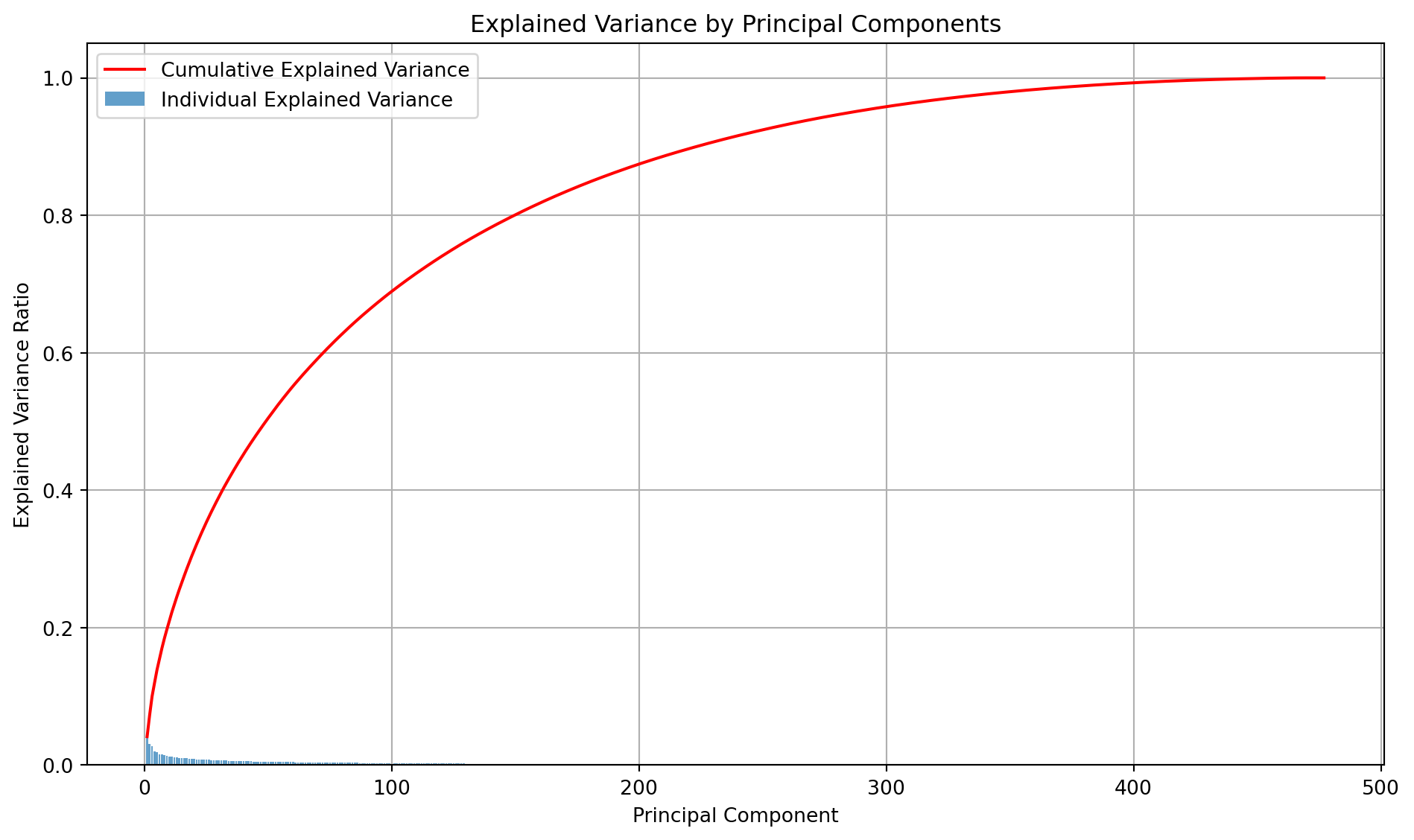

Classification model

A support vector machine classification model with an RBF kernel has been selected. A linear kernel was tested and showed poor accuracy, suggesting the data might be non-linear. The class weight option is set to balanced to enable cost-sensitive training, handling the known imbalance in the dataset.

# Create the full pipeline
pipeline_svm = Pipeline([
    ('pca', PCA()),
    ('clf', SVC(kernel="rbf", probability=True, class_weight="balanced", random_state=RANDOM_STATE))
])

Tune hyperparameters

A GradientSearchCV with 10 folds is used for the tuning of the hyperparameters. I tune both the PCA and SVM parameters simultaneously. For PCA, the fraction of explained variance is the parameter of interest. For SVM, the regularisation parameter C and the reach of influence, gamma, were the tuned parameters. It was found that the search favoured higher values of C, resulting in more complex decision boundaries and overfitting of the training data. Therefore, C was limited to a maximum value of 0.5.

# Hyperparameter tuning with GridSearchCV
print("Setting up and running GridSearchCV for hyperparameter tuning of SVM")

# Define the parameter grid
param_grid_svm = {
    "pca__n_components": [0.6, 0.7, 0.8], # Fraction values represent the fraction of variance to capture
    "clf__C": [0.1, 0.5], # Force the model to be simpler by limiting the max value of C
    "clf__gamma": [1, 0.1, 0.01, 0.001]
}

# Set up GridSearchCV scoring by Matthews CC
gs_svm = GridSearchCV(
    pipeline_svm,
    param_grid_svm,
    cv=10,
    scoring="matthews_corrcoef",
    n_jobs=-1
)

# Train the model
gs_svm.fit(X_train_mfp, y_train)

# Get the best model and parameters
svm_best_model = gs_svm.best_estimator_
svm_best_params = gs_svm.best_params_

print("\nGridSearchCV training complete.")
print(f"Best cross-validation MCC score: {gs_svm.best_score_:.4f}")
print("Best parameters found:")
print(gs_svm.best_params_)

Setting up and running GridSearchCV for hyperparameter tuning of SVM

GridSearchCV training complete.
Best cross-validation MCC score: 0.5420
Best parameters found:
{'clf__C': 0.5, 'clf__gamma': 0.1, 'pca__n_components': 0.7}

Evaluate model

After finding the best hyperparameters, the next step is to perform some evaluations of the model. First, I start with cross-validation to assess the model using only the training data before moving on to using the external validation dataset.

Helper functions

This section contains the helper functions created to assist in the evaluation tasks.

def print_metrics(metrics):
    """
    """
    formatted_metrics = {
        "AUC": f"   {round(metrics['AUC'], 4)}",
        "ACC(%)": f"{metrics['ACC'] * 100:.2f}",
        "SEN(%)": f"{metrics['SEN'] * 100:.2f}",
        "SPE(%)": f"{metrics['SPE'] * 100:.2f}",
        "MCC": f"   {round(metrics['MCC'], 4)}"
    }

    print("Performance Metrics:")
    for key, value in formatted_metrics.items():
        print(f"{key}: {value}")

    return formatted_metrics    

def run_cross_validate(model, X_train, y_train, label):
    """
    Function to perform cross-validation and plot learning curves.

    :param model: Model to validate.
    :param X_train: Training data.
    :param y_train: TRaining labels.
    :param label: Label for figure.
    :return: None
    """
    # Define stratified k-fold cross-validation
    cv = StratifiedKFold(n_splits=10,shuffle=True, random_state=1)

    # Generate learning curve data
    train_sizes, train_scores, test_scores = learning_curve(
        model, X_train, y_train, cv=cv, scoring="matthews_corrcoef",
        train_sizes=np.linspace(0.1, 1.0, 10), n_jobs=-1
    )

    # Calculate mean and standard deviation
    train_scores_mean = np.mean(train_scores, axis=1)
    test_scores_mean = np.mean(test_scores, axis=1)
    train_scores_std = np.std(train_scores, axis=1)
    test_scores_std = np.std(test_scores, axis=1)

    # Plot the learning curve
    plt.figure(figsize=(10, 6))
    plt.title(f"Learning Curve for {label}")
    plt.xlabel("Training Set Size")
    plt.ylabel("Matthews Correlation Coefficient")
    plt.grid(True)

    # Plot with shaded standard deviation
    plt.fill_between(train_sizes, train_scores_mean - train_scores_std,
                     train_scores_mean + train_scores_std, alpha=0.1, color="r")
    plt.fill_between(train_sizes, test_scores_mean - test_scores_std,
                     test_scores_mean + test_scores_std, alpha=0.1, color="g")

    plt.plot(train_sizes, train_scores_mean, "o-", color="r", label="Training score")
    plt.plot(train_sizes, test_scores_mean, "o-", color="g", label="Cross-validation score")

    plt.legend(loc="best")
    plt.tight_layout()
    
    # Save the figure
    plt.savefig(f"images/{label}_learning_curve.png")

def calculate_optimal_threshold(model, X_train, y_train):
    """
    Calculates the optimal threshold for a model using training data
    and cross-validation by finding the intersection of the sensitivity
    and specificity curves.

    :param model: Model object.
    :param X_train: Input data.
    :param y_train: Labels.
    :return: The threshold were the sensitivity and specificity curves
             intersect.
    """
    # Function to compute sensitivity and specificity
    def sen_spe(y_true, y_pred):
        cm = confusion_matrix(y_true, y_pred)
        tn, fp, fn, tp = cm.ravel()
        sen = tp / (tp + fn) if (tp + fn) > 0 else 0
        spe = tn / (tn + fp) if (tn + fp) > 0 else 0
        return sen, spe

    # Function to evaluate metrics across a range of thresholds
    def evaluate_thresholds(y_true, y_probs, thresholds=np.arange(0.0, 1.01, 0.01)):
        metrics = {"thresholds": [], "sensitivity": [], "specificity": []}

        for thresh in thresholds:
            y_pred = (y_probs >= thresh).astype(int)
            sen, spe = sen_spe(y_true, y_pred)
            metrics["thresholds"].append(thresh)
            metrics["sensitivity"].append(sen)
            metrics["specificity"].append(spe)

        return metrics

    # Set up cross-validation
    cv = StratifiedKFold(n_splits=10, shuffle=True, random_state=1)
    
    # Get out-of-fold probability predictions
    y_proba_cv = cross_val_predict(model, X_train, y_train, cv=cv, method="predict_proba", n_jobs=-1)[:, 1]

    # Get performance metrics for all thresholds
    perf_metrics = evaluate_thresholds(y_train, y_proba_cv)

    # Find the threshold where recall and specificity are closest
    differences = np.abs([a - b for a, b in zip(perf_metrics["sensitivity"], perf_metrics["specificity"])])
    intersection_index = np.argmin(differences)
    intersection_threshold = perf_metrics["thresholds"][intersection_index]
    intersection_value = perf_metrics["sensitivity"][intersection_index]

    # Plot recall and specificity curves
    plt.figure(figsize=(10, 6))
    plt.plot( perf_metrics["thresholds"], perf_metrics["sensitivity"], label="Sensitivity", color="blue")
    plt.plot( perf_metrics["thresholds"], perf_metrics["specificity"], label="Specificity", color="green")
    plt.axvline(x=intersection_threshold, color="red", linestyle="--", label=f"Intersection @ {intersection_threshold:.2f}")
    plt.scatter(intersection_threshold, intersection_value, color='red')
    plt.title("Sensitivity and Specificity vs Threshold")
    plt.xlabel("Threshold")
    plt.ylabel("Value")
    plt.legend()
    plt.grid(True)
    plt.savefig("images/recall_specificity_intersection.png")
    plt.show()

    # Print the intersection threshold
    print(f"The threshold where sensitivity and specificity intersect is approximately {intersection_threshold:.2f}")
    return intersection_threshold

def predict_with_threshold(model, data, threshold=0.5):
    """
    Predicts the label of data using a trained model and threshold.

    :param model: Model object.
    :param data: Data for prediction.
    :param threshold: Probability threshold.
    :return: Predicted label.
    """
    probs = model.predict_proba(data)[:, 1]
    return (probs >= threshold).astype(int)

def evaluate_performance(model, X_test, y_test, optimal_threshold=0.5):
    """
    Evaluates the performance of the model on test data.

    :param model: Model object.
    :param X_test: Test data.
    :param y_test: True labels.
    :param optimal_threshold: Probability threshold.
    :return: None
    """
    # Make predictions on the test set
    y_pred_probs = model.predict_proba(X_test)[:, 1] # Probabilities for the positive class
    y_predictions = predict_with_threshold(model, X_test, optimal_threshold)

    # Calculate performance metrics
    final_metrics = calculate_metrics(y_test, y_predictions, y_pred_probs)

    # Print performance metrics
    final_metrics_formatted = print_metrics(final_metrics)

    return final_metrics_formatted

def plot_roc_curve(model, X, y_true, model_name="", data_set_name=""):
    """
    Function to plot Receiver Operating Curve

    :param model: Model object.
    :param X: Data for prediction.
    :param y_true: True binary labels.
    :param model_name: Model name for labelling.
    :param data_set_name: Dataset name for labelling.
    :return: ROC data
    """
    y_probs = model.predict_proba(X)[:, 1] # Probabilities for the positive class
    
    fpr, tpr, thresholds = roc_curve(y_true, y_probs)
    auc_score = roc_auc_score(y_true, y_probs)

    # Store for plotting later
    roc_data = {'fpr': fpr, 'tpr': tpr, 'auc': auc_score}

    plt.figure(figsize=(8, 6))
    plt.plot(fpr, tpr, color="cyan", lw=2, label=f"{model_name} (AUC = {auc_score:.4f})")
    plt.plot([0, 1], [0, 1], color="black", lw=2, linestyle="--")
    plt.xlim([0.0, 1.0])
    plt.ylim([0.0, 1.05])
    plt.xlabel("False Positive Rate")
    plt.ylabel("True Positive Rate")
    plt.title(f"ROC curve on {data_set_name}")
    plt.legend(loc="lower right")
    plt.grid(alpha=0.3)
    plt.savefig("images/this_roc_curve.png")
    plt.show()

    return roc_data

def subsampling_stability_test(best_params, X_train_full, y_train_full, X_test, y_test):
    """
    This function performs a stability test on a model by repeatedly randomly sampling
    a subset of the training data, fitting the model and evaluating the performance using
    the test set. This allows for the variability in the model performance to be studied.

    :param best_params: Best parameters found from grid search.
    :param X_train_full: Full training data
    :param y_train_full: Full training labels.
    :param X_test: Test data.
    :param y_test: Test labels.
    :return: None.
    """
    # More than one thread caused issues with hanging.
    os.environ["OMP_NUM_THREADS"] = "1"

    # Define number of iterations
    n_iterations = 50
    metrics = {'AUC': [], 'ACC': [], 'SEN': [], 'SPE': [], 'MCC': []}

    # Build pipeline with best parameters
    base_pipeline = Pipeline([
        ('pca', PCA(n_components=best_params['pca__n_components'])),
        ('svm', SVC(kernel="rbf", probability=True, class_weight="balanced",
                    random_state=RANDOM_STATE, C=best_params['clf__C'],
                    gamma=best_params['clf__gamma']))
    ])

    # Run subsampling stability test
    for i in range(n_iterations):
        # Clone base pipeline
        sub_pipeline = clone(base_pipeline)
    
        # Sample 80% of training data
        X_sub, _, y_sub, _ = train_test_split(X_train_full, y_train_full,
                                              train_size=0.8, stratify=y_train_full,
                                              random_state=i)
        # Train SVM model
        sub_pipeline.fit(X_sub, y_sub)

        # Predict on test set
        y_pred = predict_with_threshold(sub_pipeline, X_test, 0.21)
        y_prob = sub_pipeline.predict_proba(X_test)[:, 1]
        single_metric = calculate_metrics(y_test, y_pred, y_prob)

        # Compute metrics
        metrics["AUC"].append(single_metric["AUC"])
        metrics["ACC"].append(single_metric["ACC"])
        metrics["SEN"].append(single_metric["SEN"])
        metrics["SPE"].append(single_metric["SPE"])
        metrics["MCC"].append(single_metric["MCC"])

    # Convert metrics to DataFrame
    metrics_df = pd.DataFrame(metrics)

    # Create side-by-side boxplots
    plt.figure(figsize=(10, 6))
    metrics_df.boxplot(column=list(metrics.keys()))
    plt.title("Metric Distributions Across Subsamples")
    plt.ylabel("Score")
    plt.grid(True)
    plt.savefig("images/metric_distributions.png")
    plt.show()

    # Calculate IQRs
    iqrs = metrics_df.quantile(0.75) - metrics_df.quantile(0.25)

    # Display the IQRs
    iqr_values = iqrs.to_dict()

    # Extract metric names and corresponding IQRs
    metrics = list(iqr_values.keys())
    values = list(iqr_values.values())

    # Create the bar plot
    plt.figure(figsize=(10, 6))
    bars = plt.bar(metrics, values, color="skyblue")
    plt.title("IQRs of Metrics from Stability Test")
    plt.xlabel("Metric")
    plt.ylabel("Interquartile Range (IQR)")
    plt.ylim(0, max(values) + 0.02)

    # Annotate bars with IQR values
    for bar, value in zip(bars, values):
        plt.text(bar.get_x() + bar.get_width() / 2,
                 bar.get_height() + 0.002, f"{value:.3f}",
                 ha="center", va="bottom")

    # Save the plot
    plt.tight_layout()
    plt.savefig("images/iqr_bar_plot.png")
    plt.show()

Cross-validation

A stratified 10-fold cross-validation was used to incrementally train the model on larger portions of the training data to generate a plot of the learning curve to diagnose the model’s performance. The resulting plot shows the model’s score (specifically, the Matthews Correlation Coefficient) on both the training set and the validation set as a function of the training set size.

The model performs exceptionally well on the data it was trained on, with the training score being consistently high. Indicating that the model has no trouble learning from the training examples. The steady increase in the cross-validation score suggests that the model is showing signs of generalisation. As it’s exposed to more data, it learns some of the underlying patterns. However, the persistent gap between the training and validation scores does indicate the model could be overfitting.

run_cross_validate(svm_best_model, X_train_mfp, y_train, "FP+PCA+SVM")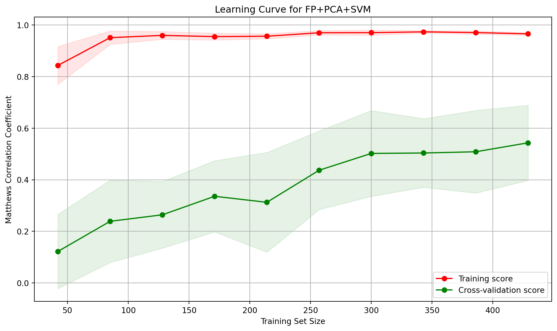

Probability threshold moving

For some classification problems that have a class imbalance, the default threshold can result in poor performance. A simple approach to improving the performance of a classifier that predicts probabilities on an imbalanced classification problem is to tune the threshold used to map probabilities to class labels.

The function calculate_optimal_threshold finds an optimal classification threshold by balancing sensitivity and specificity. Using stratified cross-validation on the training data, it generates out-of-sample probability predictions for each data point. It then iterates through a range of possible thresholds (from 0.0 to 1.0) and calculates the sensitivity and specificity for each one. The function identifies the optimal threshold as the point where the values of sensitivity and specificity are closest to each other, effectively finding the intersection of their curves. The threshold at the intersection point is returned for use in the evaluation stage.

svm_opt_thres = calculate_optimal_threshold(svm_best_model, X_train_mfp, y_train)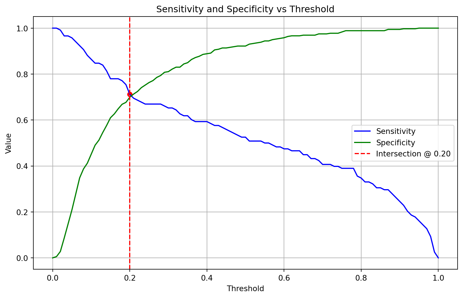

The threshold where sensitivity and specificity intersect is approximately 0.20

Evaluate model on external validation set

I now use the model to predict class labels for the external validation step. The same performance metrics as in Part 1 are used.

my_metrics = evaluate_performance(svm_best_model, X_test_mfp, y_test, svm_opt_thres)
my_metrics = {'Model': 'FP+PCA+SVM', **my_metrics}

Performance Metrics:
AUC:    0.9185
ACC(%): 82.50
SEN(%): 83.33
SPE(%): 82.22
MCC:    0.5985

Model stability check

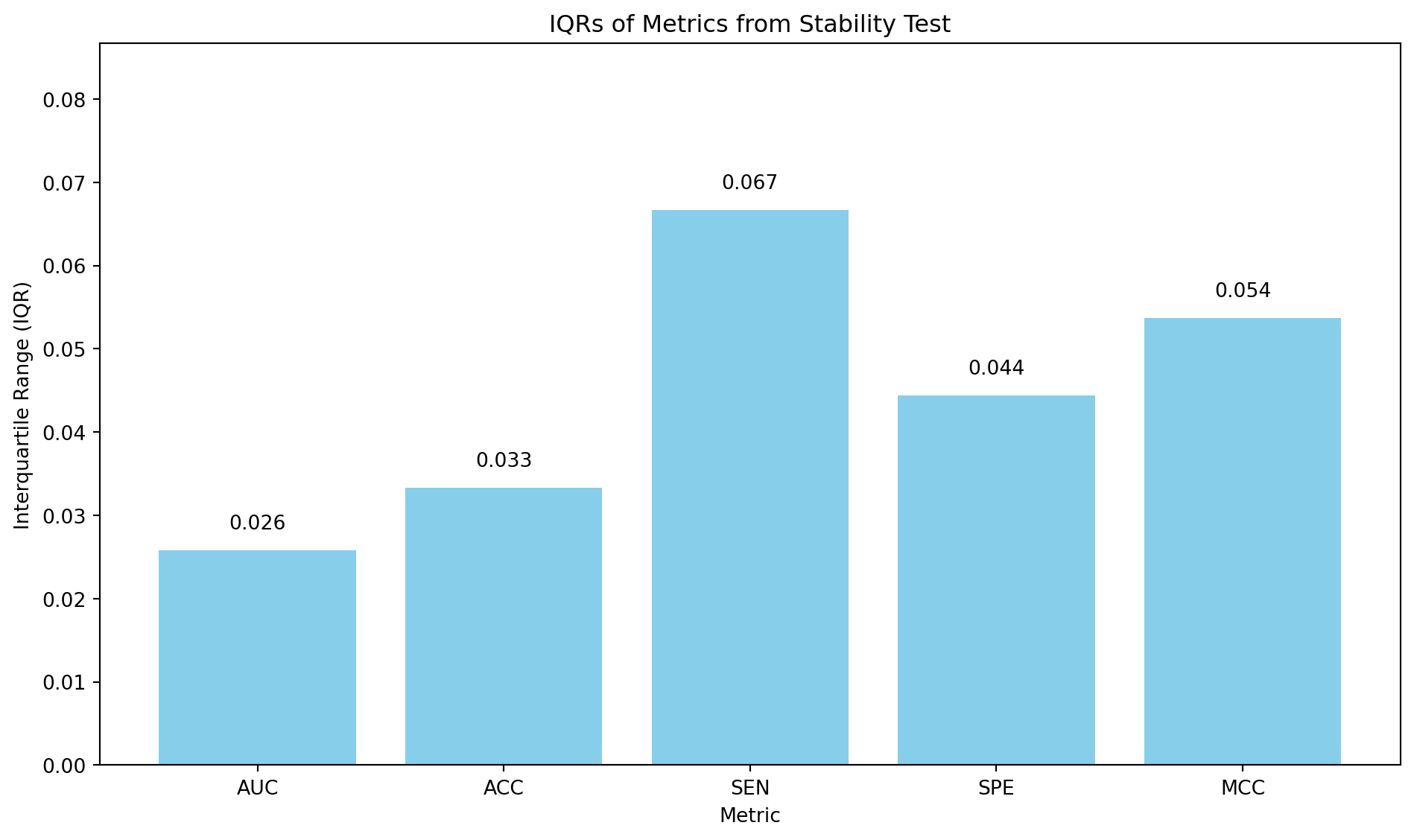
In the cross-validation stage, the learning curve suggested the model may be suffering from over-fitting. However, the model showed excellent performance on the unseen external validation data. To reveal the models’ consistency, a subsampling stability test was performed. The subsampling_stability_test function assesses the stability and robustness of the model by running a loop for a set number of iterations (50). In each iteration, the function randomly samples and trains the model on a slightly different subset (80%) of the complete training data. It then evaluates the performance of each newly trained model on the external validation set. After all iterations are completed, the performance metrics are aggregated, and their distributions are visualised using boxplots. A bar chart of the interquartile ranges (IQRs) for each metric is also produced.

The area under the curve (AUC) and accuracy (ACC) are the most stable metrics, with the lowest IQRs, indicating that the model’s overall ability to distinguish between classes and its general correctness are pretty consistent, even when trained on different subsets of the data. This is a positive sign for the model’s general reliability. The least stable metric is the sensitivity (SEN), which isn’t surprising since the dataset is imbalanced. This result shows that, whilst efforts were taken to minimise the effect of the dataset imbalance, it still does influence the model’s performance.

subsampling_stability_test(svm_best_params, X_train_mfp, y_train, X_test_mfp, y_test)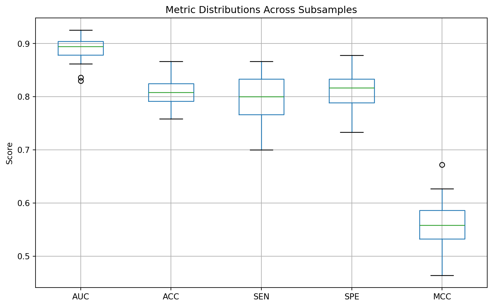

ROC curve

svm_roc = plot_roc_curve(svm_best_model, X_test_mfp, y_test, model_name="FP+PCA+SVM",
               data_set_name="Evaluation set")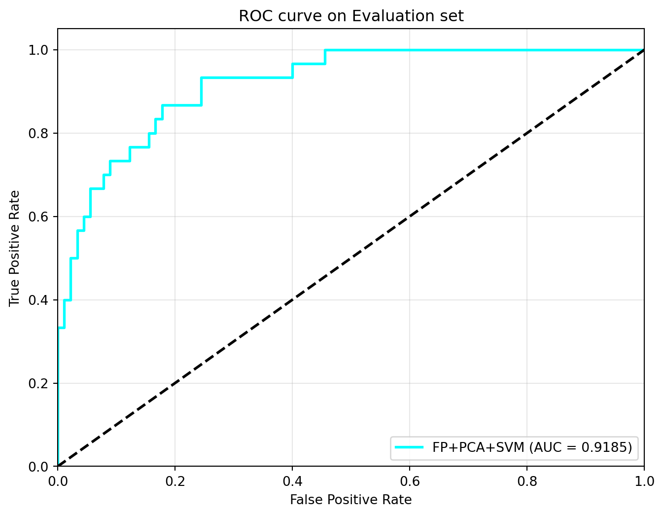

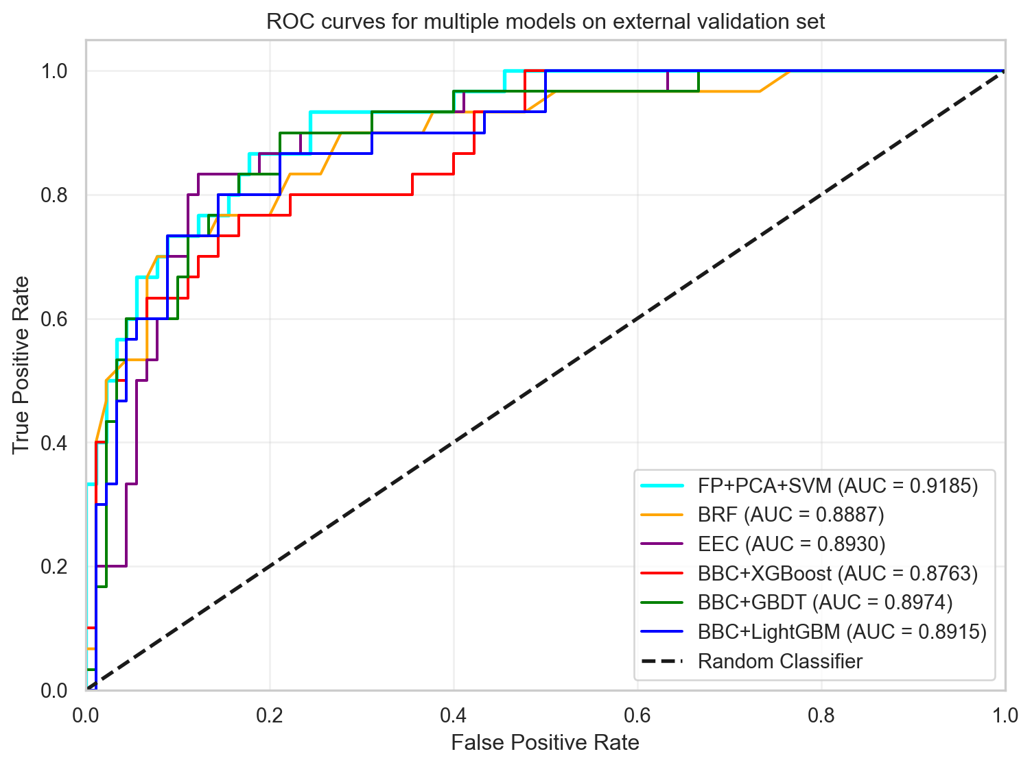
Comparison with paper

In this section, the results from FP+PCA+SVM are compared with those from the paper discussed in part 1. Comparison of the AUC and ACC metrics shows that the FP+PCA+SVM model outperforms the best model (EEC) from the paper for the AUC and is just slightly lower than EEC in accuracy (ACC). The ROC curves for each model in part 1 are combined with the FP+PCA+SVM model for visual comparison.

def create_latex_tables_compare(orig, new):
    """
    Function to combine results into a table for exporting to Latex for reporting.

    :param orig: Dictionary containing original values from the journal paper.
    :param new: Dictionary of values generated in this notebook.
    :return: None
    """
    columns = ["Model"] + METRIC_NAMES

    # New results
    df_new = pd.DataFrame([new])

    # Create a list of rows for the combined table
    rows = []
    for model, metrics in orig.items():
        external_values = metrics.get("External set", [])
        if external_values:
            row = [model] + [str(f) for f in external_values] 
            rows.append(row)
                
    # Create DataFrame of original results
    df_orig = pd.DataFrame(rows, columns=columns)

    # Combine new with original
    df_combined = pd.concat([df_new, df_orig], ignore_index=True)
                            
    # Generate LaTeX code
    latex_code = df_combined.to_latex(index=False, escape=True)

    # Save to file to include in report
    with open(f"compare_model_metrics.tex", "w") as f:
        f.write(latex_code)

    return df_combined

results = create_latex_tables_compare(original_values["RDKit_GA_65"], my_metrics)
print(results.to_string(index=False))

       Model       AUC ACC(%) SEN(%) SPE(%)       MCC
  FP+PCA+SVM    0.9185  82.50  83.33  82.22    0.5985
         BRF    0.8878  80.83  76.67  82.22    0.5444
         EEC     0.893   85.0  83.33  85.56    0.6413
 BBC+XGBoost    0.8763  80.83  73.33  83.33    0.5313
    BBC+GBDT    0.8974   85.0  73.33  88.89    0.6093
BBC+LightGBM    0.8915  84.17  73.33  87.78    0.5926

import seaborn as sns

# Set the style
sns.set_theme(style="whitegrid")

this_model = "FP+PCA+SVM"

results['Model'] = results['Model'].astype(str)
results['AUC'] = results['AUC'].astype(float)
results['ACC(%)'] = results['ACC(%)'].astype(float)

# Create subplots
fig, axes = plt.subplots(2, 1, figsize=(10, 8), sharex=True)

# Create colour palettes for highlighting the best model
colours = ["gold" if model == this_model else "skyblue" for model in results["Model"]]

# Plot AUC
sns.barplot(x='Model', y='AUC', data=results, palette=colours, ax=axes[0])
axes[0].set_title("AUC Comparison")
axes[0].set_ylabel("AUC")
axes[0].annotate("This Model", xy=(results["Model"].tolist().index(this_model), results["AUC"].max()), 
                 xytext=(0, 0.02), textcoords="offset points", ha='center', color='black')

# Plot ACC
sns.barplot(x="Model", y="ACC(%)", data=results, palette=colours)
axes[1].set_title("Accuracy (ACC%) Comparison")
axes[1].set_ylabel("Accuracy (%)")
axes[1].set_xticklabels(results["Model"], rotation=45, ha='right')
axes[1].annotate("This Model", xy=(results["Model"].tolist().index(this_model),
                                   results["ACC(%)"].iloc[results["Model"].tolist().index(this_model)]), 
                 xytext=(0, 1), textcoords="offset points", ha="center", color="black")

# Adjust layout and save the figure
plt.tight_layout()
plt.savefig("images/model_comparison_subplots.png")
plt.show()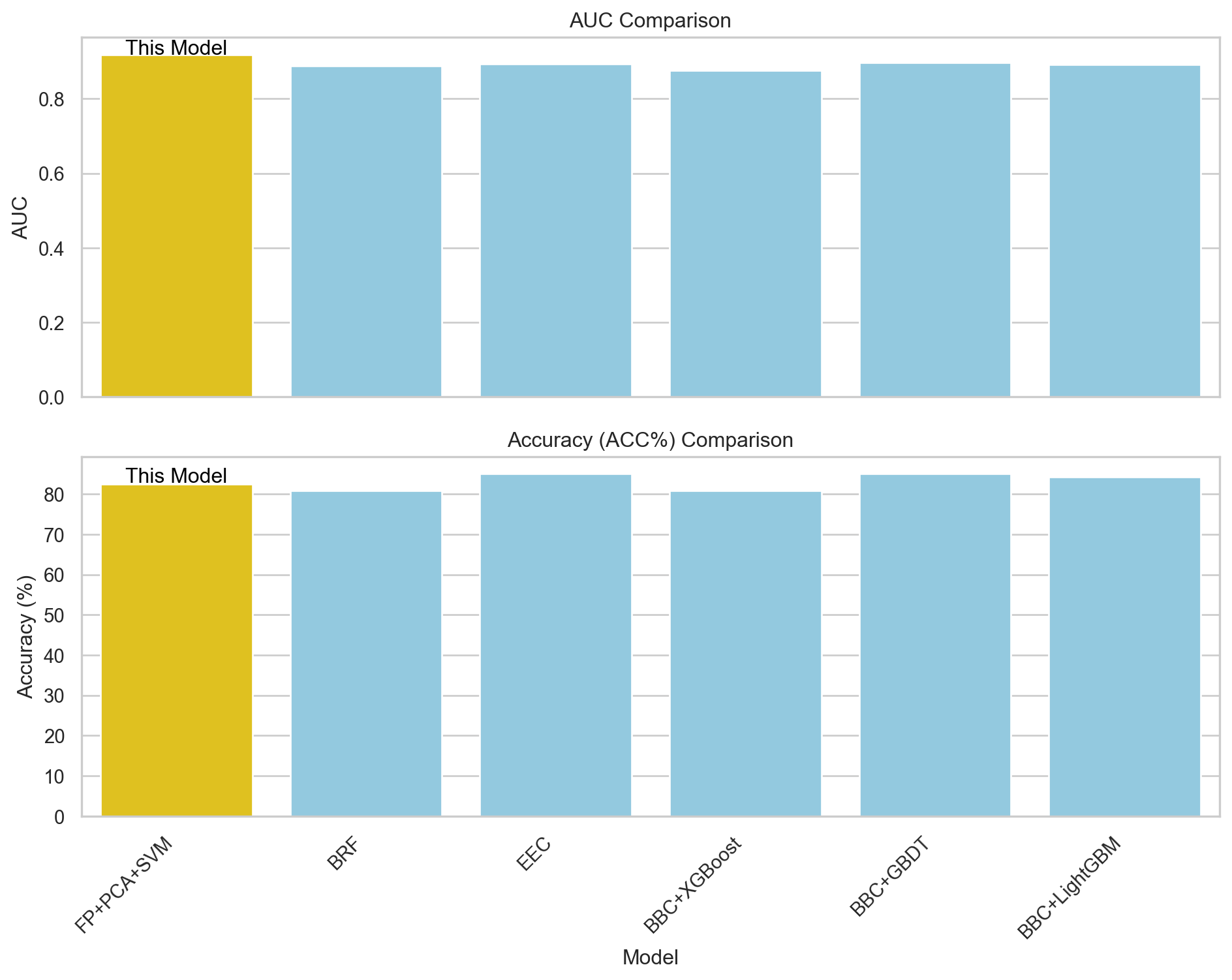

model_roc_data = roc_data["RDKit_GA_65"]

plt.figure(figsize=(8, 6))

plt.plot(svm_roc['fpr'], svm_roc['tpr'], color="cyan", lw=2,
         label=f"FP+PCA+SVM (AUC = {svm_roc['auc']:.4f})")

colours = {"BRF": "orange", "EEC": "purple", "BBC+XGBoost": "red", "BBC+GBDT": "green",
           "BBC+LightGBM": "blue"}
for model_name, data in model_roc_data.items():
    plt.plot(data["fpr"], data["tpr"], color=colours[model_name],
             label=f"{model_name} (AUC = {data['auc']:.4f})")

plt.plot([0, 1], [0, 1], "k--", lw=2, label="Random Classifier")
plt.xlim([0.0, 1.0])
plt.ylim([0.0, 1.05])
plt.title("ROC curves for multiple models on external validation set")
plt.xlabel("False Positive Rate")
plt.ylabel("True Positive Rate")
plt.legend(loc="lower right")
plt.grid(alpha=0.3)
plt.tight_layout()
plt.savefig("images/roc_curves.png")
plt.show()