import pandas as pd
import matplotlib.pyplot as plt
import seaborn as snsData Wrangling
Introduction
This task involves undertaking several data wrangling steps, including loading data, identifying missing values, handling inconsistent and missing data, aggregating the data into useful summary statistics, data transformation (feature encoding), and scaling data.
Data
The dataset used in this notebook is the Microclimate sensors data from the City of Melbourne. The data is licensed under CC BY, allowing it to be freely used for this exercise. The dataset contains climate readings from sensors located within the city of Melbourne.
Load data
The data is loaded into a pandas dataframe from the downloaded CSV file. After loading the data, the first five rows of the dataframe are inspected using the head() function.
# Load the data file into a dataframe
climate_df = pd.read_csv("microclimate-sensors-data.csv", comment="#")

# Inspect the head of the data
print(climate_df.head())
print()
Device_id Time \
0 ICTMicroclimate-08 2025-02-09T11:54:37+11:00
1 ICTMicroclimate-11 2025-02-09T12:02:11+11:00
2 ICTMicroclimate-05 2025-02-09T12:03:24+11:00
3 ICTMicroclimate-01 2025-02-09T12:02:43+11:00
4 ICTMicroclimate-09 2025-02-09T12:17:37+11:00
SensorLocation \
0 Swanston St - Tram Stop 13 adjacent Federation...
1 1 Treasury Place
2 Enterprize Park - Pole ID: COM1667
3 Birrarung Marr Park - Pole 1131
4 SkyFarm (Jeff's Shed). Rooftop - Melbourne Con...
LatLong MinimumWindDirection AverageWindDirection \
0 -37.8184515, 144.9678474 0.0 153.0
1 -37.812888, 144.9750857 0.0 144.0
2 -37.8204083, 144.9591192 0.0 45.0
3 -37.8185931, 144.9716404 NaN 150.0
4 -37.8223306, 144.9521696 0.0 241.0
MaximumWindDirection MinimumWindSpeed AverageWindSpeed GustWindSpeed \
0 358.0 0.0 3.9 7.9
1 356.0 0.0 2.0 7.8
2 133.0 0.0 1.5 2.7
3 NaN NaN 1.6 NaN
4 359.0 0.0 0.9 4.4
AirTemperature RelativeHumidity AtmosphericPressure PM25 PM10 \
0 23.9 57.300000 1009.7 0.0 0.0
1 24.5 56.200000 1005.3 0.0 0.0
2 25.0 60.000000 1009.6 1.0 3.0
3 23.1 61.099998 1009.0 0.0 5.0
4 25.6 53.700000 1007.9 0.0 0.0
Noise
0 80.500000
1 62.900000
2 68.500000
3 51.700001
4 60.200000
Inspect the data for missing values
The isnull() function is used to identify cells in the dataframe with missing or NaN values. These are summed to calculate the total number of missing values for each feature. To understand the distribution of missing data across sensors, the dataframe was also grouped by sensor device ID before calculating the sum of the missing values.
# Check how many null values in the data frame
print("Feature Name           Number of missing entries")
print(climate_df.isnull().sum())
Feature Name Number of missing entries
Device_id 0
Time 0
SensorLocation 6143
LatLong 11483
MinimumWindDirection 39343
AverageWindDirection 503
MaximumWindDirection 39501
MinimumWindSpeed 39501
AverageWindSpeed 503
GustWindSpeed 39501
AirTemperature 503
RelativeHumidity 503
AtmosphericPressure 503
PM25 18779
PM10 18779
Noise 18779
dtype: int64# Group the data by the Device_id and then sum the null values to understand the distribution of missing data across devices.
climate_df.groupby("Device_id").agg(lambda x: x.isnull().sum())| Time | SensorLocation | LatLong | MinimumWindDirection | AverageWindDirection | MaximumWindDirection | MinimumWindSpeed | AverageWindSpeed | GustWindSpeed | AirTemperature | RelativeHumidity | AtmosphericPressure | PM25 | PM10 | Noise | |
|---|---|---|---|---|---|---|---|---|---|---|---|---|---|---|---|
| Device_id | |||||||||||||||
| ICTMicroclimate-01 | 0 | 107 | 107 | 39026 | 28 | 39026 | 39026 | 28 | 39026 | 28 | 28 | 28 | 28 | 28 | 28 |
| ICTMicroclimate-02 | 0 | 108 | 108 | 16 | 16 | 16 | 16 | 16 | 16 | 16 | 16 | 16 | 16 | 16 | 16 |
| ICTMicroclimate-03 | 0 | 107 | 107 | 41 | 41 | 41 | 41 | 41 | 41 | 41 | 41 | 41 | 41 | 41 | 41 |
| ICTMicroclimate-04 | 0 | 9 | 9 | 3 | 3 | 3 | 3 | 3 | 3 | 3 | 3 | 3 | 3 | 3 | 3 |
| ICTMicroclimate-05 | 0 | 0 | 0 | 10 | 10 | 10 | 10 | 10 | 10 | 10 | 10 | 10 | 10 | 10 | 10 |
| ICTMicroclimate-06 | 0 | 107 | 107 | 8 | 8 | 8 | 8 | 8 | 8 | 8 | 8 | 8 | 8 | 8 | 8 |
| ICTMicroclimate-07 | 0 | 107 | 107 | 10 | 10 | 10 | 10 | 10 | 10 | 10 | 10 | 10 | 10 | 10 | 10 |
| ICTMicroclimate-08 | 0 | 103 | 103 | 5 | 5 | 5 | 5 | 5 | 5 | 5 | 5 | 5 | 5 | 5 | 5 |
| ICTMicroclimate-09 | 0 | 107 | 107 | 8 | 8 | 8 | 8 | 8 | 8 | 8 | 8 | 8 | 8 | 8 | 8 |
| ICTMicroclimate-10 | 0 | 4695 | 9390 | 64 | 70 | 70 | 70 | 70 | 70 | 70 | 70 | 70 | 70 | 70 | 70 |
| ICTMicroclimate-11 | 0 | 645 | 1290 | 152 | 304 | 304 | 304 | 304 | 304 | 304 | 304 | 304 | 304 | 304 | 304 |
| aws5-0999 | 0 | 48 | 48 | 0 | 0 | 0 | 0 | 0 | 0 | 0 | 0 | 0 | 18276 | 18276 | 18276 |
Data Imputation
From the above data inspections, it is observed that some features have significant missing data, e.g. PM25, PM10 and Noise for device aws5-0999. The values for certain features should be constant, such as sensor location, latitude and longitude, making the correction of missing data for them easier. Whereas the values of other features are based on measurement, and therefore, the correction of missing data will require some assumptions and computations.
SensorLocation
The number of unique sensor locations for each device is one, confirming the assumption that each sensor is in a fixed location. Therefore, the existing values can be used to correct any missing values in the dataset. To correct the missing sensor locations, I grouped the data by Device_id and then selected the SensorLocation column using only the first entry in each group. The first entry in each group is then used in a map command to replace the missing sensor locations.
# Get the number of unique locations for each sensor.
num_locations = climate_df.groupby("Device_id")[["SensorLocation"]].nunique()
print("Number of unique sensor locations for each device:", num_locations)
Number of unique sensor locations for each device: SensorLocation
Device_id
ICTMicroclimate-01 1
ICTMicroclimate-02 1
ICTMicroclimate-03 1
ICTMicroclimate-04 1
ICTMicroclimate-05 1
ICTMicroclimate-06 1
ICTMicroclimate-07 1
ICTMicroclimate-08 1
ICTMicroclimate-09 1
ICTMicroclimate-10 1
ICTMicroclimate-11 1
aws5-0999 1# Create sensor location mapping for each device
device_location_map = climate_df.groupby("Device_id")[["SensorLocation"]].first()
# Apply the device location map to correct the missing sensor locations
climate_df["SensorLocation"] = climate_df["Device_id"].map(device_location_map["SensorLocation"])
# Check the number of missing sensor locations after correction
print("Number of missing sensor locations values:", climate_df["SensorLocation"].isnull().sum())Number of missing sensor locations values: 0LatLong
The same approach used to correct the SensorLocation is used for the LatLong. First, I check that each device only has one unique value, then I retrieve the valid value for each device and use it to correct the missing values.
# Get the number of unique latitude/longitude locations for each sensor.
num_latlong = climate_df.groupby("Device_id")[["LatLong"]].nunique()
print("Number of unique sensor latitude/longitude locations for each device:")
print(num_locations)
Number of unique sensor latitude/longitude locations for each device:
SensorLocation
Device_id
ICTMicroclimate-01 1
ICTMicroclimate-02 1
ICTMicroclimate-03 1
ICTMicroclimate-04 1
ICTMicroclimate-05 1
ICTMicroclimate-06 1
ICTMicroclimate-07 1
ICTMicroclimate-08 1
ICTMicroclimate-09 1
ICTMicroclimate-10 1
ICTMicroclimate-11 1
aws5-0999 1# Create lat/long mapping for each device
device_latlong_map = climate_df.groupby("Device_id")[["LatLong"]].first()
# Apply the device lat/long map to correct the missing sensor latitudes and longitudes
climate_df["LatLong"] = climate_df["Device_id"].map(device_latlong_map["LatLong"])
# Check the number of missing LatLong values after correction
print("Number of missing sensor latitude/logitude values:", climate_df["LatLong"].isnull().sum())Number of missing sensor latitude/logitude values: 0Continuous features
Inconsistent data
Before making any corrections to the continuous features, it is a good idea to inspect some basic statistics.
climate_df.describe()| MinimumWindDirection | AverageWindDirection | MaximumWindDirection | MinimumWindSpeed | AverageWindSpeed | GustWindSpeed | AirTemperature | RelativeHumidity | AtmosphericPressure | PM25 | PM10 | Noise | |
|---|---|---|---|---|---|---|---|---|---|---|---|---|
| count | 352450.000000 | 391290.000000 | 352292.000000 | 352292.000000 | 391290.000000 | 352292.000000 | 391290.000000 | 391290.000000 | 391290.000000 | 373014.000000 | 373014.000000 | 373014.000000 |
| mean | 20.447147 | 166.414570 | 305.508777 | 4.794662 | 1.058048 | 3.441384 | 16.378137 | 66.467364 | 1002.152184 | 20.116674 | 8.138810 | 66.417315 |
| std | 57.606792 | 125.167169 | 89.833971 | 38.599842 | 0.980283 | 2.607634 | 6.075031 | 18.367640 | 108.405272 | 118.284124 | 12.522434 | 13.052584 |
| min | 0.000000 | 0.000000 | 0.000000 | 0.000000 | 0.000000 | 0.000000 | -0.800000 | 4.000000 | 20.900000 | 0.000000 | 0.000000 | 0.000000 |
| 25% | 0.000000 | 43.000000 | 314.000000 | 0.000000 | 0.400000 | 1.500000 | 12.100000 | 55.100000 | 1008.800000 | 1.000000 | 3.000000 | 59.000000 |
| 50% | 0.000000 | 159.000000 | 353.000000 | 0.000000 | 0.800000 | 2.800000 | 15.900000 | 68.200000 | 1014.700000 | 3.000000 | 5.000000 | 68.300000 |
| 75% | 0.000000 | 301.000000 | 358.000000 | 0.100000 | 1.500000 | 4.800000 | 19.800000 | 79.600000 | 1020.100000 | 7.000000 | 9.000000 | 72.400000 |
| max | 359.000000 | 359.000000 | 360.000000 | 359.000000 | 11.100000 | 52.500000 | 40.800000 | 99.800003 | 1042.900000 | 1030.700000 | 308.000000 | 131.100000 |
From the above table, there appears to be some issue with the MinimumWindSpeed, AtmosphericPressure and PM25.
- MinimumWindSpeed: The maximum minimum wind speed value is 359 m/s. This is not sensible and beyond the upper bound (60 m/s) of the instrument’s measurement range.
- AtmosphericPressure: The minimum atmospheric pressure value of 20.9 hPa is too low.
- PM25: The maximum value of 1030.7 is beyond the measurement range of the instrument (0-1000 micrograms/m^3).
To inspect further, I calculated the descriptive statistics for each device.
# Calculate the min, max, mean and standard deviation for each device, only for the MinimumWindSpeed, AtmosphericPressure, and PM25 features
climate_df.groupby("Device_id")[["MinimumWindSpeed", "AtmosphericPressure", "PM25"]].agg(["min", "max", "mean", "std"])| MinimumWindSpeed | AtmosphericPressure | PM25 | ||||||||||
|---|---|---|---|---|---|---|---|---|---|---|---|---|
| min | max | mean | std | min | max | mean | std | min | max | mean | std | |
| Device_id | ||||||||||||
| ICTMicroclimate-01 | NaN | NaN | NaN | NaN | 991.400024 | 1040.300049 | 1015.682445 | 8.009809 | 0.0 | 235.0 | 5.278630 | 11.171503 |
| ICTMicroclimate-02 | 0.0 | 11.4 | 0.577927 | 0.871374 | 987.300000 | 1036.000000 | 1011.590638 | 7.957121 | 1.0 | 147.0 | 7.800387 | 9.512505 |
| ICTMicroclimate-03 | 0.0 | 10.1 | 0.725178 | 0.824416 | 986.400000 | 1035.200000 | 1010.733407 | 7.959522 | 1.0 | 184.0 | 6.979975 | 8.255256 |
| ICTMicroclimate-04 | 0.0 | 1.7 | 0.001496 | 0.024614 | 996.700000 | 1037.900000 | 1018.512888 | 7.243488 | 0.0 | 81.0 | 5.085106 | 7.566532 |
| ICTMicroclimate-05 | 0.0 | 7.8 | 0.197126 | 0.360950 | 993.600000 | 1037.700000 | 1015.707429 | 7.856305 | 1.0 | 116.0 | 6.684698 | 8.098758 |
| ICTMicroclimate-06 | 0.0 | 0.8 | 0.002879 | 0.027912 | 992.100000 | 1040.900000 | 1016.449209 | 7.983454 | 0.0 | 92.0 | 5.183268 | 8.530823 |
| ICTMicroclimate-07 | 0.0 | 1.1 | 0.000896 | 0.018917 | 994.300000 | 1042.900000 | 1018.497433 | 8.014416 | 0.0 | 62.0 | 5.542080 | 7.993104 |
| ICTMicroclimate-08 | 0.0 | 1.5 | 0.004890 | 0.048268 | 991.900000 | 1040.900000 | 1016.326436 | 8.032214 | 0.0 | 98.0 | 7.447921 | 9.736321 |
| ICTMicroclimate-09 | 0.0 | 0.4 | 0.000449 | 0.009074 | 990.700000 | 1039.700000 | 1015.006325 | 7.896735 | 0.0 | 307.0 | 7.610188 | 24.851515 |
| ICTMicroclimate-10 | 0.0 | 359.0 | 56.584262 | 123.228729 | 20.900000 | 1030.700000 | 838.528264 | 363.300887 | 0.0 | 1030.7 | 188.700070 | 389.082039 |
| ICTMicroclimate-11 | 0.0 | 359.0 | 6.172891 | 46.169169 | 32.700000 | 1029.700000 | 994.319084 | 125.177193 | 0.0 | 1024.1 | 21.611508 | 133.095076 |
| aws5-0999 | 0.0 | 4.4 | 0.415397 | 0.466901 | 989.700000 | 1038.700000 | 1015.150175 | 8.420255 | NaN | NaN | NaN | NaN |
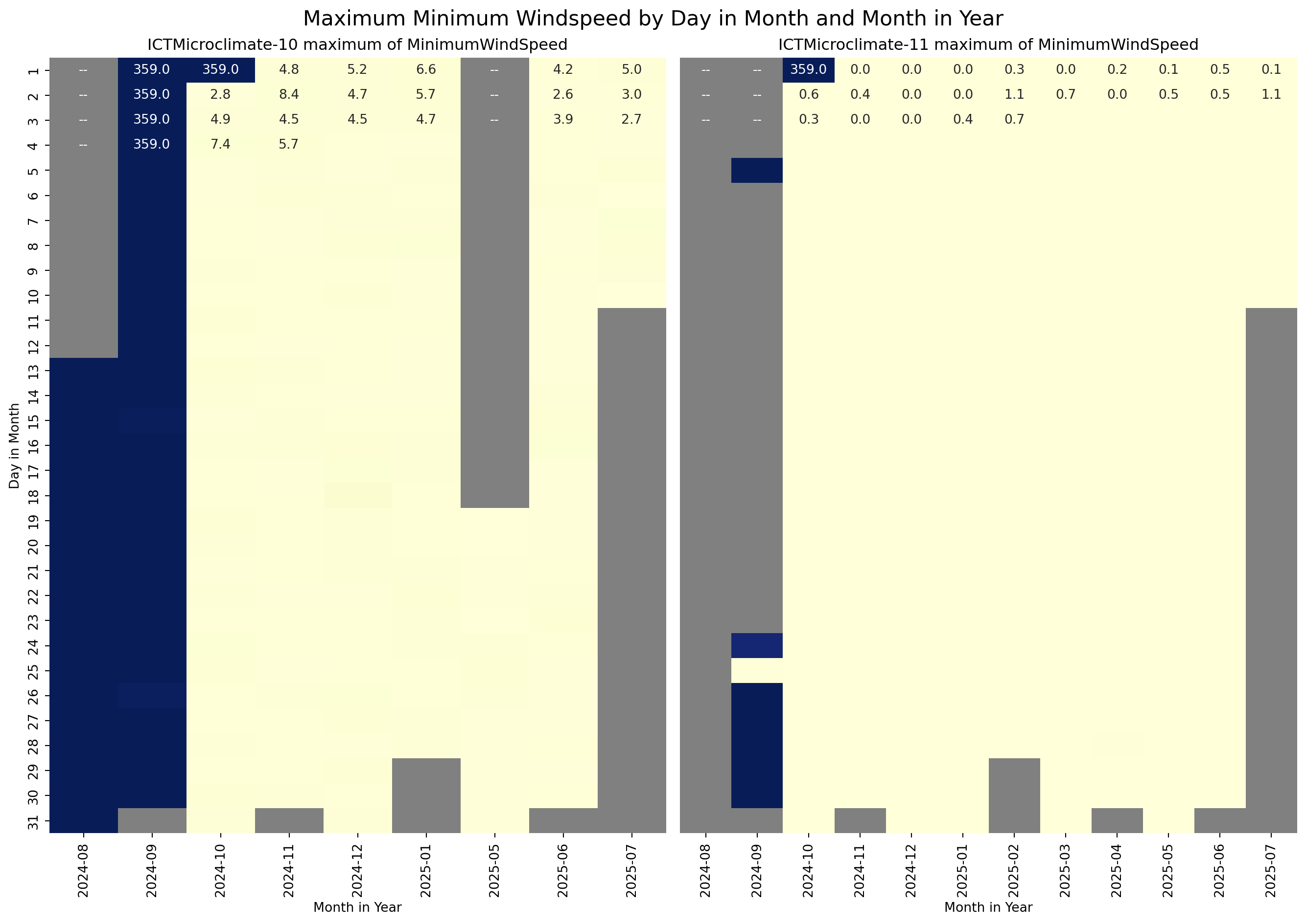
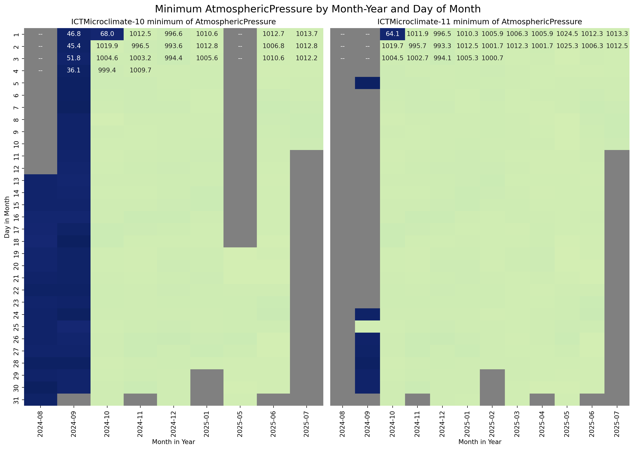
Inspection of the statistics for each device shows that the problematic values only occur for the ICTMicroclimate-10 and ICTMicroclimate-11 sensors, which are both at the same location, Treasury Place.
climate_df.groupby("Device_id")[["SensorLocation"]].first().iloc[-3:-1]| SensorLocation | |
|---|---|
| Device_id | |
| ICTMicroclimate-10 | 1 Treasury Place |
| ICTMicroclimate-11 | 1 Treasury Place |
The next step is to visualise the temporal distribution of the MinimumWindSpeed, AtmosphericPressure, and PM25 for the ICTMicroclimate-10 and ICTMicroclimate-11 sensors to see if the inconsistent values were random or followed a pattern. For the visualisation, I used a heatmap of Day in the Month versus Month in the Year.
# Ensure Time is datetime
climate_df["Time"] = pd.to_datetime(climate_df["Time"], utc=True)

# Drop timezone information
climate_df["Time"] = climate_df["Time"].dt.tz_localize(None)

# Extract year-month and hour
climate_df["year_month"] = climate_df["Time"].dt.to_period("M").astype(str)
climate_df["day"] = climate_df["Time"].dt.day

# Extract groups ICTMicroclimate-10 and ICTMicroclimate-11 as DataFrames
d_10_df = climate_df.groupby("Device_id").get_group("ICTMicroclimate-10")
d_11_df = climate_df.groupby("Device_id").get_group("ICTMicroclimate-11")

# Group by year_month and hour, and get max windspeed
g_10 = d_10_df.groupby(["day","year_month", ])["MinimumWindSpeed"].max().unstack()
g_11 = d_11_df.groupby(["day","year_month", ])["MinimumWindSpeed"].max().unstack()

# Set common colour scale limits
vmin = 0
vmax = 360

# Create subplots
fig, axes = plt.subplots(1, 2, figsize=(14, 10), sharey=True)

cmap = plt.cm.YlGnBu
cmap.set_bad(color="grey")

# Plot heatmap
sns.heatmap(g_10, ax=axes[0], annot=True, fmt=".1f", cmap=cmap, vmin=vmin, vmax=vmax, cbar=False)
axes[0].set_title("ICTMicroclimate-10 maximum of MinimumWindSpeed")
axes[0].set_ylabel("Day in Month")
axes[0].set_xlabel("Month in Year")

# Plot heatmap
sns.heatmap(g_11, ax=axes[1], vmin=vmin, vmax=vmax, annot=True, fmt=".1f", cmap=cmap, cbar=False)
axes[1].set_title("ICTMicroclimate-11 maximum of MinimumWindSpeed")
axes[1].set_ylabel("")
axes[1].tick_params(left=False)
axes[1].set_xlabel("Month in Year")

# Add a title to the entire figure
fig.suptitle("Maximum Minimum Windspeed by Day in Month and Month in Year", fontsize=16)

plt.tight_layout()
plt.show()
C:\Users\darrin\anaconda3\Lib\site-packages\seaborn\matrix.py:260: FutureWarning:
Format strings passed to MaskedConstant are ignored, but in future may error or produce different behavior
C:\Users\darrin\anaconda3\Lib\site-packages\seaborn\matrix.py:260: FutureWarning:
Format strings passed to MaskedConstant are ignored, but in future may error or produce different behavior
# Group by year_month and hour, and get min AtmosphericPressure
g_10 = d_10_df.groupby(["day","year_month", ])["AtmosphericPressure"].min().unstack()
g_11 = d_11_df.groupby(["day","year_month", ])["AtmosphericPressure"].min().unstack()

# Set common color scale limits
vmin = 0
vmax = 1300

# Create subplots
fig, axes = plt.subplots(1, 2, figsize=(14, 10), sharey=True)

cmap = plt.cm.YlGnBu_r
cmap.set_bad(color="grey")

# Plot heatmap
sns.heatmap(g_10, ax=axes[0], annot=True, fmt=".1f", cmap=cmap, vmin=vmin, vmax=vmax, cbar=False)
axes[0].set_title("ICTMicroclimate-10 minimum of AtmosphericPressure")
axes[0].set_ylabel("Day in Month")
axes[0].set_xlabel("Month in Year")

# Plot heatmap
sns.heatmap(g_11, ax=axes[1], vmin=vmin, vmax=vmax, annot=True, fmt=".1f", cmap=cmap, cbar=False)
axes[1].set_title("ICTMicroclimate-11 minimum of AtmosphericPressure")
axes[1].set_ylabel("")
axes[1].tick_params(left=False)
axes[1].set_xlabel("Month in Year")

# Add a title to the entire figure
fig.suptitle("Minimum AtmosphericPressure by Month-Year and Day of Month", fontsize=16)

plt.tight_layout()
plt.show()
C:\Users\darrin\anaconda3\Lib\site-packages\seaborn\matrix.py:260: FutureWarning:
Format strings passed to MaskedConstant are ignored, but in future may error or produce different behavior
C:\Users\darrin\anaconda3\Lib\site-packages\seaborn\matrix.py:260: FutureWarning:
Format strings passed to MaskedConstant are ignored, but in future may error or produce different behavior
# Group by year_month and hour, and get min AtmosphericPressure
g_10 = d_10_df.groupby(["day","year_month", ])["PM25"].max().unstack()
g_11 = d_11_df.groupby(["day","year_month", ])["PM25"].max().unstack()

# Set common colour scale limits
vmin = 0
vmax = 1300

# Create subplots
fig, axes = plt.subplots(1, 2, figsize=(14, 10), sharey=True)

cmap = plt.cm.YlGnBu
cmap.set_bad(color="grey")

# Plot heatmap
sns.heatmap(g_10, ax=axes[0], annot=True, fmt=".1f", cmap=cmap, vmin=vmin, vmax=vmax, cbar=False)
axes[0].set_title("ICTMicroclimate-10 maximum of PM25")
axes[0].set_ylabel("Day in Month")
axes[0].set_xlabel("Month in Year")

# Plot heatmap
sns.heatmap(g_11, ax=axes[1], vmin=vmin, vmax=vmax, annot=True, fmt=".1f", cmap=cmap, cbar=False)
axes[1].set_title("ICTMicroclimate-11 maximum of PM25")
axes[1].set_ylabel("")
axes[1].tick_params(left=False)
axes[1].set_xlabel("Month in Year")

# Add a title to the entire figure
fig.suptitle("Maximum PM25 by Month-Year and Day of Month", fontsize=16)

plt.tight_layout()
plt.show()
C:\Users\darrin\anaconda3\Lib\site-packages\seaborn\matrix.py:260: FutureWarning:
Format strings passed to MaskedConstant are ignored, but in future may error or produce different behavior
C:\Users\darrin\anaconda3\Lib\site-packages\seaborn\matrix.py:260: FutureWarning:
Format strings passed to MaskedConstant are ignored, but in future may error or produce different behavior
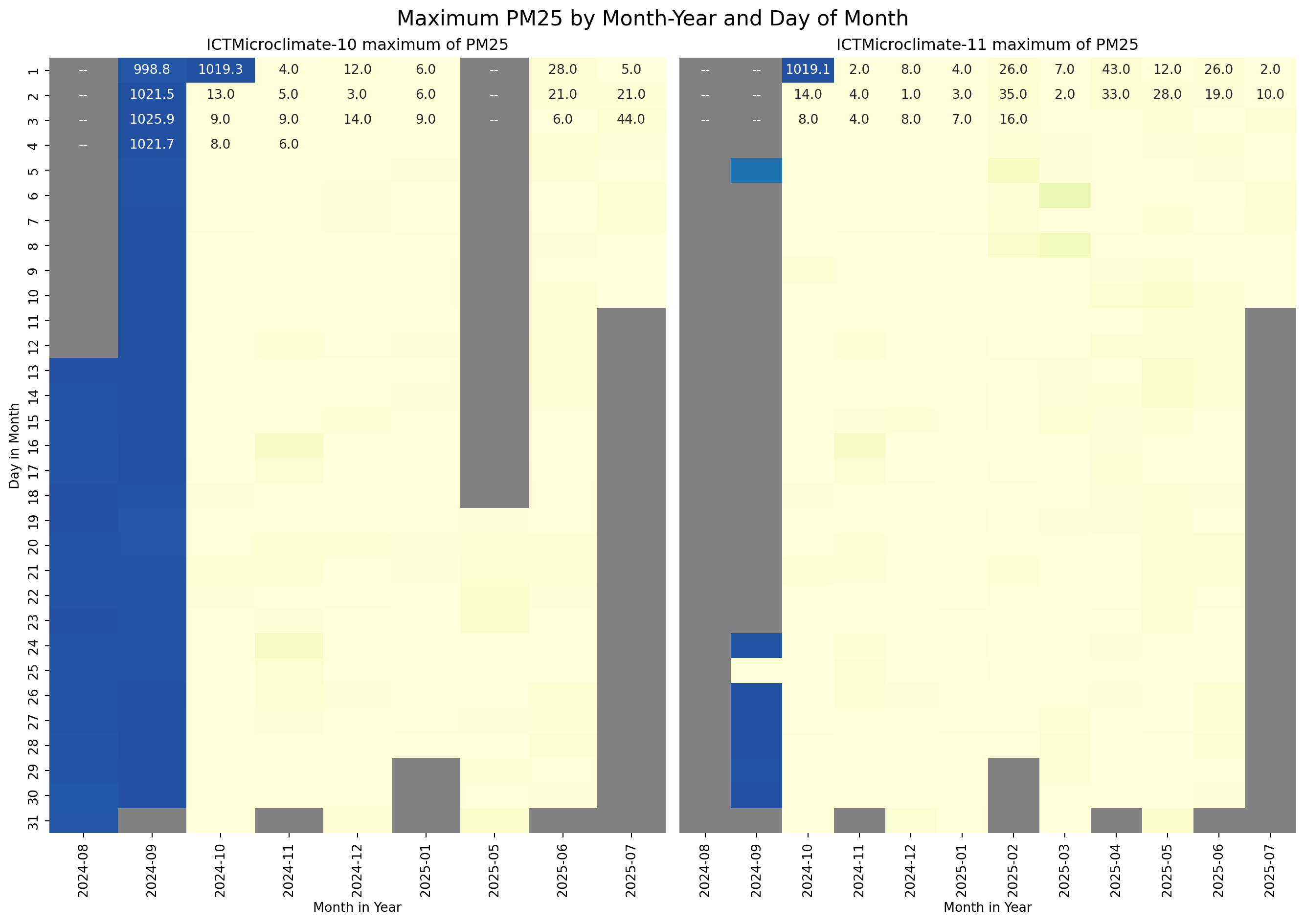
From the above plots, it is clear that the data for sensors ICTMicroclimate-10 and ICTMicroclimate-11 is unreliable from August 2024 until the 2nd of October 2024. For the purposes of this exercise, the data for these sensors during this period will be removed from the dataframe.
# Define the device and time range to filter out
devices_to_remove = ["ICTMicroclimate-10","ICTMicroclimate-11"]
end_time = "2024-10-01 23:59:59"

# Filter out rows for that device in the given time range
df_filtered = climate_df[~((climate_df["Device_id"].isin(devices_to_remove)) & (climate_df["Time"] <= end_time))].copy()

df_filtered.groupby("Device_id")[["MinimumWindSpeed", "AtmosphericPressure", "PM25"]].agg(["min", "max", "mean", "std"])

# Drop the columns created for the above plotting
df_filtered.drop(columns=["day","year_month"], inplace=True)

# Calculate the min, max, mean and standard deviation for each device, only for the MinimumWindSpeed, AtmosphericPressure, and PM25 features
df_filtered.groupby("Device_id")[["MinimumWindSpeed", "AtmosphericPressure", "PM25"]].agg(["min", "max", "mean", "std"])| MinimumWindSpeed | AtmosphericPressure | PM25 | ||||||||||
|---|---|---|---|---|---|---|---|---|---|---|---|---|
| min | max | mean | std | min | max | mean | std | min | max | mean | std | |
| Device_id | ||||||||||||
| ICTMicroclimate-01 | NaN | NaN | NaN | NaN | 991.400024 | 1040.300049 | 1015.682445 | 8.009809 | 0.0 | 235.0 | 5.278630 | 11.171503 |
| ICTMicroclimate-02 | 0.0 | 11.4 | 0.577927 | 0.871374 | 987.300000 | 1036.000000 | 1011.590638 | 7.957121 | 1.0 | 147.0 | 7.800387 | 9.512505 |
| ICTMicroclimate-03 | 0.0 | 10.1 | 0.725178 | 0.824416 | 986.400000 | 1035.200000 | 1010.733407 | 7.959522 | 1.0 | 184.0 | 6.979975 | 8.255256 |
| ICTMicroclimate-04 | 0.0 | 1.7 | 0.001496 | 0.024614 | 996.700000 | 1037.900000 | 1018.512888 | 7.243488 | 0.0 | 81.0 | 5.085106 | 7.566532 |
| ICTMicroclimate-05 | 0.0 | 7.8 | 0.197126 | 0.360950 | 993.600000 | 1037.700000 | 1015.707429 | 7.856305 | 1.0 | 116.0 | 6.684698 | 8.098758 |
| ICTMicroclimate-06 | 0.0 | 0.8 | 0.002879 | 0.027912 | 992.100000 | 1040.900000 | 1016.449209 | 7.983454 | 0.0 | 92.0 | 5.183268 | 8.530823 |
| ICTMicroclimate-07 | 0.0 | 1.1 | 0.000896 | 0.018917 | 994.300000 | 1042.900000 | 1018.497433 | 8.014416 | 0.0 | 62.0 | 5.542080 | 7.993104 |
| ICTMicroclimate-08 | 0.0 | 1.5 | 0.004890 | 0.048268 | 991.900000 | 1040.900000 | 1016.326436 | 8.032214 | 0.0 | 98.0 | 7.447921 | 9.736321 |
| ICTMicroclimate-09 | 0.0 | 0.4 | 0.000449 | 0.009074 | 990.700000 | 1039.700000 | 1015.006325 | 7.896735 | 0.0 | 307.0 | 7.610188 | 24.851515 |
| ICTMicroclimate-10 | 0.0 | 10.5 | 0.711077 | 0.889946 | 989.700000 | 1028.900000 | 1010.033453 | 7.718326 | 0.0 | 85.0 | 5.132205 | 7.261089 |
| ICTMicroclimate-11 | 0.0 | 1.6 | 0.008341 | 0.060927 | 989.500000 | 1029.700000 | 1010.929081 | 7.414035 | 0.0 | 179.0 | 3.857938 | 6.942787 |
| aws5-0999 | 0.0 | 4.4 | 0.415397 | 0.466901 | 989.700000 | 1038.700000 | 1015.150175 | 8.420255 | NaN | NaN | NaN | NaN |
The table above shows some descriptive statistics for the MinimumWindSpeed, AtmosphericPressure, and PM25 features after filtering out the corrupted data for sensors ICTMicroclimate-10 and ICTMicroclimate-11. It is observed that the previosuly identified issues are no longer present.
Missing data
The task description requires the use of either the mean or the median to fill in missing values. The median is the best choice for distributions that are skewed or contain outliers. Therefore, I’ll plot the distributions of all variables to decide if the median or mean should be used.
# Get list of features to plot
float_features = df_filtered.select_dtypes(include='number').columns.tolist()

# Plot histograms using the pandas hist() function
axes = df_filtered.hist(column=float_features, bins=15,layout=(8,2), figsize=(10,15), edgecolor="white",log=True)
for ax in axes.flatten():
    ax.set_ylabel("Count (log scale)")

plt.tight_layout()
plt.show()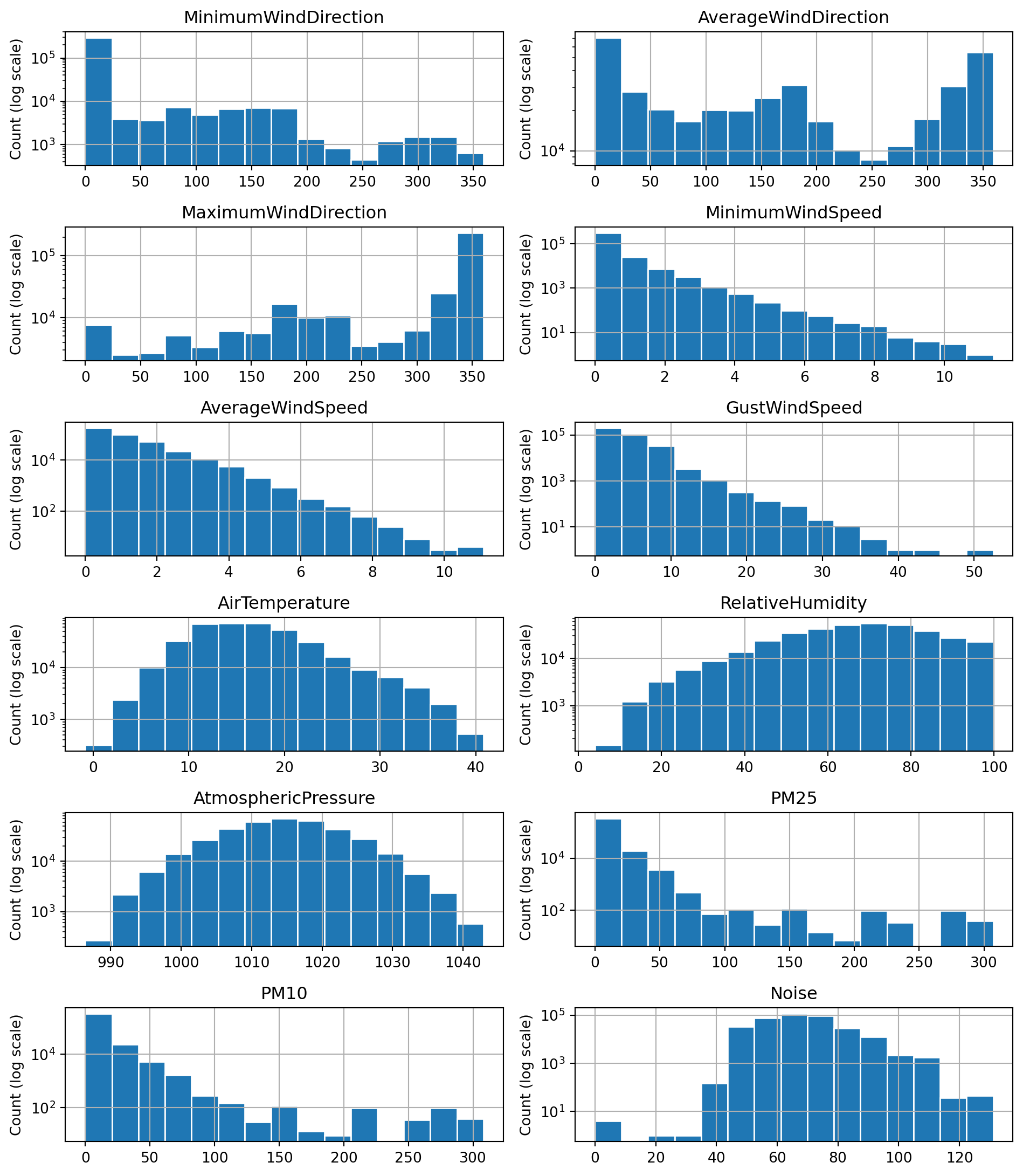
The majority of the above distributions are highly skewed or contain outliers. The distributions for AtmosphericPressure and AirTemperature are the closest to symmetric distributions. Based on this evidence, I decided to use the median value for imputing missing values as it is less affected by the skewness of a distribution.
# Calculate the median value for each feature
feature_medians = df_filtered.median(numeric_only=True)
print("Meadian values for each feature:")
print(feature_medians)

# Replace missing values in numeric feature columns with the median
df_filled = df_filtered.fillna(feature_medians)
Meadian values for each feature:
MinimumWindDirection 0.0
AverageWindDirection 159.0
MaximumWindDirection 353.0
MinimumWindSpeed 0.0
AverageWindSpeed 0.8
GustWindSpeed 2.8
AirTemperature 16.1
RelativeHumidity 68.4
AtmosphericPressure 1014.8
PM25 3.0
PM10 5.0
Noise 68.3
dtype: float64# Check how many null values in the data frame after filling missing values
print("Feature Name Number of missing entries")
print(df_filled.isnull().sum())Feature Name Number of missing entries
Device_id 0
Time 0
SensorLocation 0
LatLong 0
MinimumWindDirection 0
AverageWindDirection 0
MaximumWindDirection 0
MinimumWindSpeed 0
AverageWindSpeed 0
GustWindSpeed 0
AirTemperature 0
RelativeHumidity 0
AtmosphericPressure 0
PM25 0
PM10 0
Noise 0
dtype: int64Distributions of PM10 and PM25
The histograms of the PM10 and PM25 features are shown in the figures below. Both distributions have the shape of an exponential distribution, with high counts at low particulate matter, and the counts decreasing exponentially as the particulate matter increases.
num_bins = 10

# Create figure with specified size
hist_fig = plt.figure(figsize=(10, 7))

# Plot PM10
ax1 = plt.subplot(2, 1, 1)  # 2 rows, 1 column, 1st subplot
ax1.hist(df_filled["PM10"], num_bins, edgecolor="white", log=True)
ax1.set_title(f'Histogram of PM10 (n={df_filtered["PM10"].shape[0]})')
ax1.set_ylabel("Count (log scale)")
ax1.set_xlabel(r"Particular matter 10 $\mu m$ diameter $\left(\frac{\mu g}{m^3}\right)$")

# Plot PM25
ax2 = plt.subplot(212, sharex=ax1)  # 2 rows, 1 column, 2nd subplot
ax2.hist(df_filled["PM25"], num_bins, edgecolor="white", log=True)
ax2.set_title(f'Histogram of PM25 (n={df_filtered["PM25"].shape[0]})')
ax2.set_ylabel("Count (log scale)")
ax2.set_xlabel(r"Particulate matter 2.5 $\mu m$ diameter $\left(\frac{\mu g}{m^3}\right)$")

# Set the x limit for both plots
#plt.xlim(0, 350)

plt.tight_layout()
plt.show()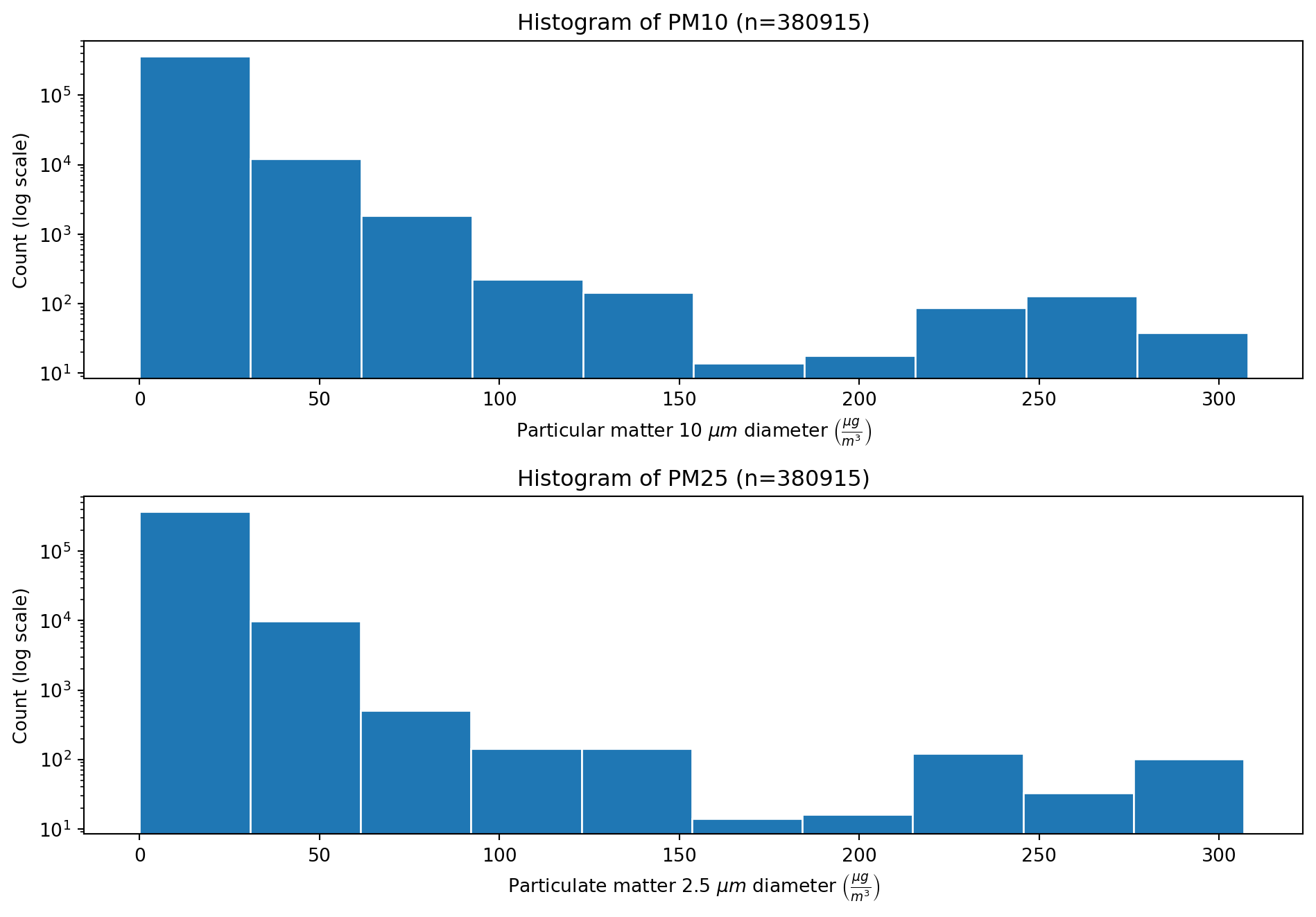
To investigate any possible correlation between the PM10 and PM25 features, a scater plot was created to allow visual inspection. Then the pearson correlation cofficient was calculated.
# Create figure with specified size
plt.figure(figsize=(10, 7))

# Scatter plot of
plt.scatter(df_filtered["PM25"], df_filtered["PM10"], s=10, edgecolor="lightskyblue", alpha=0.5)
plt.grid(zorder=1, alpha=0.5)

plt.title("Scatter plot of PM25 verus PM10")
plt.xlabel(r"Particulate matter 2.5 $\mu m$ diameter $\left(\frac{\mu g}{m^3}\right)$")
plt.ylabel(r"Particulate matter 10 $\mu m$ diameter $\left(\frac{\mu g}{m^3}\right)$")

plt.xlim(0, 350)
plt.ylim(0, 350)

plt.tight_layout()
plt.show()
# Pearson correlation coefficient
correlation = df_filled["PM25"].corr(df_filled["PM10"])
print(f"Correlation coefficient between features PM25 and PM10 is: {correlation:.3}")
Correlation coefficient between features PM25 and PM10 is: 0.985The scatter plot between the features PM25 and PM10 shows a strong positive linear relationship. This is confirmed with the high pearson correlation.
LatLong encoding
The first step in encoding the LatLong feature was to split it into the latitude and longitude components.
df_filled[['latitude', 'longitude']] = df_filled['LatLong'].str.split(',', expand=True).astype(float)The second step is to choose an encoding system. Here, I have chosen to encode the latitude and longitude into a 3D Cartesian coordinate system, giving values for x, y and z. This approximates the Earth as a sphere, which is reasonable since the region of interest is a tiny portion of the Earth’s surface. This encoding approach will enable accurate distance measurement between points if required in the machine learning algorithm.
# Converting lat/long to cartesian
import numpy as np

# Convert from degrees to radians
df_filled["lat_rad"] = np.radians(df_filled["latitude"])
df_filled["long_rad"] = np.radians(df_filled["longitude"])

# Calculate the Cartesian values
df_filled["x"] = np.cos(df_filled["lat_rad"]) * np.cos(df_filled["long_rad"])
df_filled["y"] = np.cos(df_filled["lat_rad"]) * np.sin(df_filled["long_rad"])
df_filled["z"] = np.sin(df_filled["lat_rad"])

# Drop the intermediate lat_rad and long_rad columns
df_filled.drop(columns=["lat_rad","long_rad"], inplace=True)

# Print out the encoding
print("Table showing the encoded values, x, y and z for each latitude and longitude pair.")
df_filled.groupby(['latitude','longitude'])[['x','y','z']].agg(['unique'])
Table showing the encoded values, x, y and z for each latitude and longitude pair.| x | y | z | ||
|---|---|---|---|---|
| unique | unique | unique | ||
| latitude | longitude | |||
| -37.822331 | 144.952170 | [-0.6466829154533684] | [0.45361725572202244] | [-0.6132149640802587] |
| -37.822234 | 144.982941 | [-0.6469272879344449] | [0.453270475112011] | [-0.6132136336689813] |
| -37.822183 | 144.956222 | [-0.6467162961870897] | [0.45357241883254756] | [-0.6132129264133661] |
| -37.820408 | 144.959119 | [-0.6467547756329378] | [0.4535506263400986] | [-0.6131884616840834] |
| -37.819499 | 144.978721 | [-0.6469178722458754] | [0.45333491635230483] | [-0.6131759292280787] |
| -37.818593 | 144.971640 | [-0.6468697848649976] | [0.453420426464369] | [-0.6131634352222753] |
| -37.818452 | 144.967847 | [-0.6468410076851618] | [0.45346411834148037] | [-0.6131614829338421] |
| -37.814604 | 144.970299 | [-0.6468941255968796] | [0.4534600727651171] | [-0.61310843468028] |
| -37.814035 | 144.967280 | [-0.6468752177437501] | [0.4534976554876418] | [-0.6131005864751623] |
| -37.812888 | 144.975086 | [-0.6469470430816873] | [0.45341656703589844] | [-0.6130847740608488] |
| -37.812860 | 144.974539 | [-0.6469429703681334] | [0.45342290938269164] | [-0.613084381091373] |
| -37.795617 | 144.951901 | [-0.6469147812012331] | [0.4537844284725181] | [-0.6128466026170258] |
# Drop the latitude and longitude columns
df_filled.drop(columns=["latitude","longitude","LatLong"], inplace=True)
Feature scaling
Each feature in the dataset has different scale (range). To normalise the features, min-max scaling is applied to all continuous data.
Feature distributions before scaling
Distributions of the features are plotted before scaling.
# Get list of features to plot
scale_float_features = df_filled.select_dtypes(include='number').columns.tolist()

axes = df_filled.hist(column=scale_float_features, bins=15,layout=(8,2), figsize=(10,15), edgecolor="white", xlabelsize=7, ylabelsize=7, log=True)
for ax in axes.flatten():
    ax.set_ylabel("Count (log scale)")

plt.tight_layout()
plt.show()
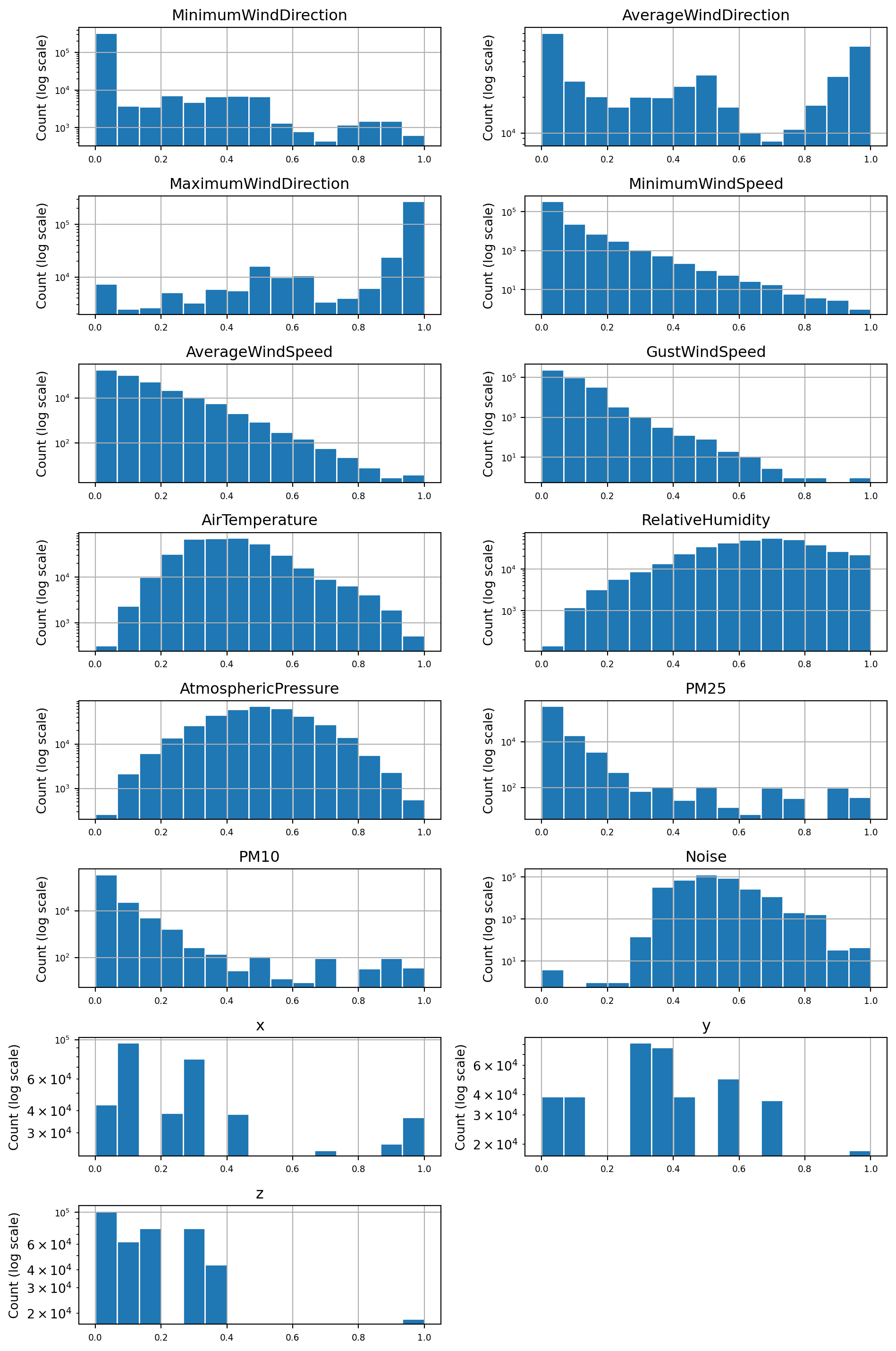
Scaling operation
# Create a copy of the filled dataframe
df_scaled = df_filled.copy()

# Apply min-max scaling to the selected columns
for feature in scale_float_features:
    min_val = df_scaled[feature].min()
    max_val = df_scaled[feature].max()
    df_scaled[feature] = (df_scaled[feature] - min_val) / (max_val - min_val)
Feature distributions after scaling
Distributions of the features plotted after scaling. Inspection of the before an after figures for each features distribution shows that the scaling did not affect the relative shape of the distribution (e.g. skewness).
# Loop through all of the continuous features, plotting their distributions
axes = df_scaled.hist(column=scale_float_features, bins=15,layout=(8,2), figsize=(10,15), edgecolor="white", xlabelsize=7, ylabelsize=7, log=True)

for ax in axes.flatten():
    ax.set_ylabel("Count (log scale)")
plt.tight_layout()
plt.show()