import pandas as pd
import numpy as np
import matplotlib.pyplot as plt
import seaborn as sns
import shap
import warnings
from collections import Counter
from imblearn.over_sampling import SMOTE
from skopt import BayesSearchCV
from sklearn.preprocessing import LabelEncoder, OneHotEncoder, StandardScaler
from sklearn.linear_model import LogisticRegression
from sklearn.model_selection import GridSearchCV, learning_curve, StratifiedKFold, StratifiedShuffleSplit, cross_val_score
from sklearn.metrics import f1_score, confusion_matrix, classification_report
from sklearn.svm import SVC
from sklearn.tree import DecisionTreeClassifier, plot_tree
from sklearn.inspection import permutation_importance

# Suppress all UserWarnings
warnings.filterwarnings("ignore", category=UserWarning)Liver Cirrhosis
Introduction
The goal of this task is to build several machine learning models for predicting the survival status of patients with liver cirrhosis. The dataset for model development and training is sourced from the Cirrhosis Patient Survival Prediction dataset in the UC Irvine Machine Learning Repository. The data is licensed under CC BY, allowing it to be freely used for this exercise. This dataset contains 17 clinical features collected from 418 patients with liver cirrhosis. The survival states included are Death (0), Censored (1), and Censored due to liver transplant (2).
Since there are three target classes, this is a multi-class classification problem. For the success measures, the following were used:
- Confusion Matrix to give a breakdown of actual vs. predicted classes.
- Precision, Recall, and F1-Score using macro averaging to treat all classes equally
- Precision: How many predicted class X are actually class X?
- Recall: How many actual class X were correctly predicted?
- F1-Score: Harmonic mean of precision and recall.
EDA
Here, I conduct the exploratory data analysis. Starting by loading the data, then exploring the data using descriptive statistics and visualisations to understand features and target variables.
# Load data
df = pd.read_csv("cirrhosis.csv")

# Inspect the head of the data
print(df.head())

# Inspect the shape of the data
print(f"\nData shape: {df.shape}")
ID N_Days Status Drug Age Sex Ascites Hepatomegaly Spiders \
0 1 400 D D-penicillamine 21464 F Y Y Y
1 2 4500 C D-penicillamine 20617 F N Y Y
2 3 1012 D D-penicillamine 25594 M N N N
3 4 1925 D D-penicillamine 19994 F N Y Y
4 5 1504 CL Placebo 13918 F N Y Y
Edema Bilirubin Cholesterol Albumin Copper Alk_Phos SGOT \
0 Y 14.5 261.0 2.60 156.0 1718.0 137.95
1 N 1.1 302.0 4.14 54.0 7394.8 113.52
2 S 1.4 176.0 3.48 210.0 516.0 96.10
3 S 1.8 244.0 2.54 64.0 6121.8 60.63
4 N 3.4 279.0 3.53 143.0 671.0 113.15
Tryglicerides Platelets Prothrombin Stage
0 172.0 190.0 12.2 4.0
1 88.0 221.0 10.6 3.0
2 55.0 151.0 12.0 4.0
3 92.0 183.0 10.3 4.0
4 72.0 136.0 10.9 3.0
Data shape: (418, 20)Drop irrelevant columns
The ID and N_Days columns are not clinical features as specified in the dataset metadata. This task involves only using the clinical features for model development.
df.drop(["ID", "N_Days"], axis=1, inplace=True)Check for missing values
Inspection for missing values reveals that some of the features are missing a significant number of entries. These will be handled in the pre-processing section.
# Check how many null values are in the data frame
print("\nFeature Name  Number of missing entries")
print(df.isnull().sum())
Feature Name  Number of missing entries
Status             0
Drug             106
Age                0
Sex                0
Ascites          106
Hepatomegaly     106
Spiders          106
Edema              0
Bilirubin          0
Cholesterol      134
Albumin            0
Copper           108
Alk_Phos         106
SGOT             106
Tryglicerides    136
Platelets         11
Prothrombin        2
Stage              6
dtype: int64
Basis statistics
Inspect the statistics of the numerical features. A value of count below 418, signifies the feature has missing values. The maximum value
df.describe()| Age | Bilirubin | Cholesterol | Albumin | Copper | Alk_Phos | SGOT | Tryglicerides | Platelets | Prothrombin | Stage | |
|---|---|---|---|---|---|---|---|---|---|---|---|
| count | 418.000000 | 418.000000 | 284.000000 | 418.000000 | 310.000000 | 312.000000 | 312.000000 | 282.000000 | 407.000000 | 416.000000 | 412.000000 |
| mean | 18533.351675 | 3.220813 | 369.510563 | 3.497440 | 97.648387 | 1982.655769 | 122.556346 | 124.702128 | 257.024570 | 10.731731 | 3.024272 |
| std | 3815.845055 | 4.407506 | 231.944545 | 0.424972 | 85.613920 | 2140.388824 | 56.699525 | 65.148639 | 98.325585 | 1.022000 | 0.882042 |
| min | 9598.000000 | 0.300000 | 120.000000 | 1.960000 | 4.000000 | 289.000000 | 26.350000 | 33.000000 | 62.000000 | 9.000000 | 1.000000 |
| 25% | 15644.500000 | 0.800000 | 249.500000 | 3.242500 | 41.250000 | 871.500000 | 80.600000 | 84.250000 | 188.500000 | 10.000000 | 2.000000 |
| 50% | 18628.000000 | 1.400000 | 309.500000 | 3.530000 | 73.000000 | 1259.000000 | 114.700000 | 108.000000 | 251.000000 | 10.600000 | 3.000000 |
| 75% | 21272.500000 | 3.400000 | 400.000000 | 3.770000 | 123.000000 | 1980.000000 | 151.900000 | 151.000000 | 318.000000 | 11.100000 | 4.000000 |
| max | 28650.000000 | 28.000000 | 1775.000000 | 4.640000 | 588.000000 | 13862.400000 | 457.250000 | 598.000000 | 721.000000 | 18.000000 | 4.000000 |
Visualisations
Numerical features
Histograms of each numerical feature are shown below. Apart from age, the other numerical features show skew (both positive and negative) and outliers.
# Get a list of the numerical columns
num_cols = df.select_dtypes(include=["float64", "int64"]).columns

custom_palette = [
    "skyblue", "salmon", "lightgreen", "orange", "violet",
    "gold", "turquoise", "lightcoral", "plum", "khaki", "mediumseagreen"
]

# Plot the numerical data
fig, axes = plt.subplots(6, 2, figsize = (8, 16))
axes = axes.flatten()

for i, col in enumerate(num_cols):
    sns.histplot(data = df[col], kde = True, ax = axes[i], color=custom_palette[i])

# Remove the unused subplot (12th axis)
for j in range(len(num_cols), len(axes)):
    fig.delaxes(axes[j])

plt.tight_layout()
plt.show()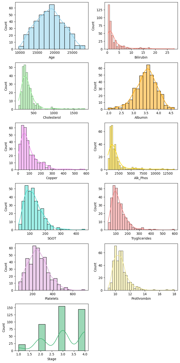
fig, axes = plt.subplots(6, 2, figsize = (8, 16))
axes = axes.flatten()

for i, col in enumerate(num_cols):
    sns.boxplot(data = df[col], ax = axes[i], color=custom_palette[i])

# Remove the unused subplot (12th axis)
for j in range(len(num_cols), len(axes)):
    fig.delaxes(axes[j])

plt.tight_layout()
plt.show()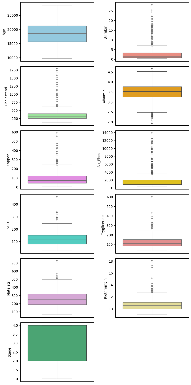
Categorical features
Bar plots of each categorical feature are shown below. Some of the feature columns are quite imbalanced, such as Sex, Ascites, Edema, and stage. The target “Status” also exhibits an imbalance between the classes.
# Get a list of categorical columns
cat_cols = df.select_dtypes(include=["object"]).columns

fig, axes = plt.subplots(4, 2, figsize = (8, 16))
axes = axes.flatten()

# Plot the categorical data
for i, col in enumerate(cat_cols):
    sns.countplot(x=df[col], data=df, hue=df[col], ax=axes[i], legend=False)

# Remove the unused subplot (12th axis)
for j in range(len(cat_cols), len(axes)):
    fig.delaxes(axes[j])

plt.tight_layout()
plt.show()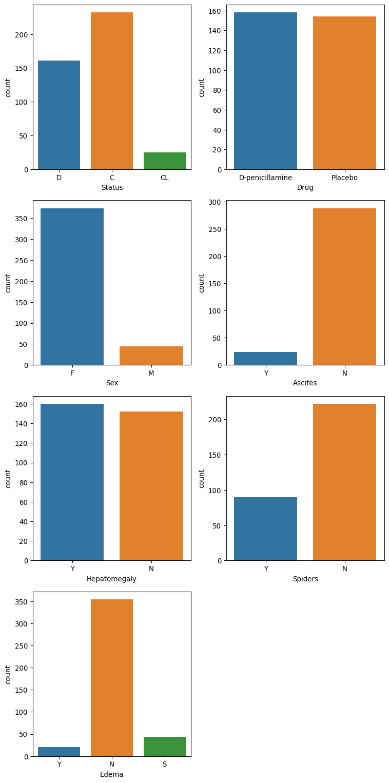
Preprocess the data
Check and remove duplicates
# Count duplicate rows
duplicate_count = df.duplicated().sum()

print(f"Number of duplicate rows: {duplicate_count}")
Number of duplicate rows: 0Handling missing values
In the EDA section, it was noted that many of the features had missing values. These occurred in both the numerical and categorical features. The imputation method used for each type is: * Numerical: Use the median to avoid the effect of outliers. * Categorical: Use the most common (mode).
# Detect and analyse missing values
missing_count = df.isnull().sum().astype(int)
missing_percentage = round(df.isnull().mean() * 100, 2)

# Create a DataFrame
missing_df = pd.DataFrame({
    "missing_count": missing_count,
    "missing_percentage": missing_percentage
})

# Check the number of missing values for the numerical features
print(missing_df.loc[num_cols])
missing_count missing_percentage
Age 0 0.00
Bilirubin 0 0.00
Cholesterol 134 32.06
Albumin 0 0.00
Copper 108 25.84
Alk_Phos 106 25.36
SGOT 106 25.36
Tryglicerides 136 32.54
Platelets 11 2.63
Prothrombin 2 0.48
Stage 6 1.44# Replacing missing values in numerical columns using the median
for col in num_cols:
df[col] = df[col].fillna(df[col].median())# Check the number of missing values is now zero.
print("\nFeature Name Number of missing entries")
print(df[num_cols].isnull().sum())
Feature Name  Number of missing entries
Age              0
Bilirubin        0
Cholesterol      0
Albumin          0
Copper           0
Alk_Phos         0
SGOT             0
Tryglicerides    0
Platelets        0
Prothrombin      0
Stage            0
dtype: int64
# Remove the "Status" from the list, as this is our target
cat_cols = cat_cols[1:]
# Check the number of missing values for the categorical features
print(missing_df.loc[cat_cols]) missing_count missing_percentage
Drug 106 25.36
Sex 0 0.00
Ascites 106 25.36
Hepatomegaly 106 25.36
Spiders 106 25.36
Edema 0 0.00for col in cat_cols:
df[col] = df[col].fillna(df[col].mode().values[0])# Check the number of missing values is now zero.
print("\nFeature Name Number of missing entries")
print(df[cat_cols].isnull().sum())
Feature Name  Number of missing entries
Drug            0
Sex             0
Ascites         0
Hepatomegaly    0
Spiders         0
Edema           0
dtype: int64
Split data into test and train
Stratified sampling has been used to ensure the class proportions remain the same in the test and train sets.
Create features and target
X_df = df.drop(["Status"], axis=1)
y_df = df["Status"]
print(f"Training shape: {X_df.shape}")
print(f"Target shape: {y_df.shape}")
Training shape: (418, 17)
Target shape: (418,)Split the data
stratSplit = StratifiedShuffleSplit(n_splits=1, test_size=0.2, random_state=0)

for train_index, test_index in stratSplit.split(X_df, y_df):
    X_train_df = X_df.iloc[train_index]
    X_test_df = X_df.iloc[test_index]
    y_train_df = y_df.iloc[train_index]
    y_test_df = y_df.iloc[test_index]

X_train_df.reset_index(drop=True, inplace=True)
X_test_df.reset_index(drop=True, inplace=True)
y_train_df.reset_index(drop=True, inplace=True)
y_test_df.reset_index(drop=True, inplace=True)
Check data types
# Numerical column types
print(f"{len(num_cols)} columns of numerical type:")
X_train_df[num_cols].dtypes
11 columns of numerical type:Age int64
Bilirubin float64
Cholesterol float64
Albumin float64
Copper float64
Alk_Phos float64
SGOT float64
Tryglicerides float64
Platelets float64
Prothrombin float64
Stage float64
dtype: object# Categorical column types
print(f"{len(cat_cols)} columns of type categorical")
X_train_df[cat_cols].dtypes6 columns of type categoricalDrug object
Sex object
Ascites object
Hepatomegaly object
Spiders object
Edema object
dtype: objectEncode categorical features
All of the categorical features can be one-hot encoded.
# Print unique values for each selected column
for column in cat_cols:
    unique_values = df[column].unique()
    print(f"Unique values in column '{column}':")
    print(unique_values)
    print("-" *70)
Unique values in column 'Drug':
['D-penicillamine' 'Placebo']
----------------------------------------------------------------------
Unique values in column 'Sex':
['F' 'M']
----------------------------------------------------------------------
Unique values in column 'Ascites':
['Y' 'N']
----------------------------------------------------------------------
Unique values in column 'Hepatomegaly':
['Y' 'N']
----------------------------------------------------------------------
Unique values in column 'Spiders':
['Y' 'N']
----------------------------------------------------------------------
Unique values in column 'Edema':
['Y' 'N' 'S']
----------------------------------------------------------------------Encoding nominal categorical features
# Columns to encode
one_hot_cols = cat_cols[:]

# OneHotEncoder setup
encoder = OneHotEncoder(sparse_output=False)
X_nom_enc_train = encoder.fit_transform(X_train_df[one_hot_cols])
X_nom_enc_test = encoder.fit_transform(X_test_df[one_hot_cols])

# Convert to DataFrame with column names
train_enc_df = pd.DataFrame(X_nom_enc_train, columns=encoder.get_feature_names_out(one_hot_cols))
test_enc_df = pd.DataFrame(X_nom_enc_test, columns=encoder.get_feature_names_out(one_hot_cols))

# Assemble training and test sets
X_train_enc_df = pd.concat([train_enc_df , X_train_df[num_cols]], axis=1)
#X_train_enc_df.info()
X_test_enc_df = pd.concat([test_enc_df , X_test_df[num_cols]], axis=1)
X_test_enc_df.head()| Drug_D-penicillamine | Drug_Placebo | Sex_F | Sex_M | Ascites_N | Ascites_Y | Hepatomegaly_N | Hepatomegaly_Y | Spiders_N | Spiders_Y | ... | Bilirubin | Cholesterol | Albumin | Copper | Alk_Phos | SGOT | Tryglicerides | Platelets | Prothrombin | Stage | |
|---|---|---|---|---|---|---|---|---|---|---|---|---|---|---|---|---|---|---|---|---|---|
| 0 | 0.0 | 1.0 | 1.0 | 0.0 | 1.0 | 0.0 | 0.0 | 1.0 | 0.0 | 1.0 | ... | 4.4 | 316.0 | 3.62 | 308.0 | 1119.0 | 114.70 | 322.0 | 282.0 | 9.8 | 4.0 |
| 1 | 1.0 | 0.0 | 1.0 | 0.0 | 1.0 | 0.0 | 1.0 | 0.0 | 1.0 | 0.0 | ... | 1.5 | 293.0 | 4.30 | 50.0 | 975.0 | 125.55 | 56.0 | 336.0 | 9.1 | 2.0 |
| 2 | 1.0 | 0.0 | 1.0 | 0.0 | 1.0 | 0.0 | 0.0 | 1.0 | 1.0 | 0.0 | ... | 7.3 | 309.5 | 3.52 | 73.0 | 1259.0 | 114.70 | 108.0 | 265.0 | 11.1 | 1.0 |
| 3 | 1.0 | 0.0 | 1.0 | 0.0 | 1.0 | 0.0 | 1.0 | 0.0 | 0.0 | 1.0 | ... | 3.8 | 426.0 | 3.22 | 96.0 | 2716.0 | 210.80 | 113.0 | 228.0 | 10.6 | 2.0 |
| 4 | 1.0 | 0.0 | 1.0 | 0.0 | 1.0 | 0.0 | 0.0 | 1.0 | 0.0 | 1.0 | ... | 1.8 | 244.0 | 2.54 | 64.0 | 6121.8 | 60.63 | 92.0 | 183.0 | 10.3 | 4.0 |
5 rows × 24 columns
Target encoding
status_mapping = {"D": 0, "C": 1, "CL": 2}

# Apply the mapping
y_train_df = y_train_df.map(status_mapping)
y_test_df = y_test_df.map(status_mapping)
Feature scaling
# Create numpy arrays using the encoded and values for the features.
X_train_enc = X_train_enc_df.to_numpy()
X_test_enc = X_test_enc_df.to_numpy()
# Fit scaler on training data
scaler = StandardScaler()
X_train = scaler.fit_transform(X_train_enc)
# Transform test data using the same scaler
X_test = scaler.transform(X_test_enc)
pd.DataFrame(X_train).describe().round(3)
pd.DataFrame(X_test).describe().round(3)| 0 | 1 | 2 | 3 | 4 | 5 | 6 | 7 | 8 | 9 | ... | 14 | 15 | 16 | 17 | 18 | 19 | 20 | 21 | 22 | 23 | |
|---|---|---|---|---|---|---|---|---|---|---|---|---|---|---|---|---|---|---|---|---|---|
| count | 84.000 | 84.000 | 84.000 | 84.000 | 84.000 | 84.000 | 84.000 | 84.000 | 84.000 | 84.000 | ... | 84.000 | 84.000 | 84.000 | 84.000 | 84.000 | 84.000 | 84.000 | 84.000 | 84.000 | 84.000 |
| mean | 0.212 | -0.212 | 0.178 | -0.178 | -0.011 | 0.011 | -0.109 | 0.109 | -0.145 | 0.145 | ... | 0.059 | 0.175 | 0.001 | 0.032 | 0.076 | 0.104 | 0.054 | 0.070 | 0.069 | -0.281 |
| std | 0.932 | 0.932 | 0.741 | 0.741 | 1.028 | 1.028 | 0.971 | 0.971 | 1.098 | 1.098 | ... | 1.132 | 1.502 | 1.029 | 0.928 | 0.950 | 0.855 | 1.162 | 0.962 | 1.162 | 1.126 |
| min | -1.253 | -0.798 | -2.750 | -0.364 | -4.072 | -0.246 | -0.773 | -1.293 | -1.978 | -0.506 | ... | -0.646 | -1.231 | -3.638 | -1.070 | -0.712 | -1.510 | -1.391 | -1.837 | -1.641 | -2.443 |
| 25% | -1.253 | -0.798 | 0.364 | -0.364 | 0.246 | -0.246 | -0.773 | -1.293 | -1.978 | -0.506 | ... | -0.553 | -0.243 | -0.355 | -0.438 | -0.270 | -0.226 | -0.401 | -0.629 | -0.728 | -1.264 |
| 50% | 0.798 | -0.798 | 0.364 | -0.364 | 0.246 | -0.246 | -0.773 | 0.773 | 0.506 | -0.506 | ... | -0.354 | -0.201 | 0.077 | -0.236 | -0.270 | -0.095 | -0.205 | -0.046 | -0.119 | -0.085 |
| 75% | 0.798 | 1.253 | 0.364 | -0.364 | 0.246 | -0.246 | 1.293 | 0.773 | 0.506 | 1.978 | ... | 0.129 | 0.063 | 0.740 | 0.089 | 0.042 | 0.348 | 0.173 | 0.627 | 0.312 | 1.094 |
| max | 0.798 | 1.253 | 0.364 | 2.750 | 0.246 | 4.072 | 1.293 | 0.773 | 0.506 | 1.978 | ... | 5.208 | 8.300 | 2.420 | 4.677 | 5.168 | 4.148 | 5.996 | 2.687 | 6.476 | 1.094 |
8 rows × 24 columns
Training set class distribution
Here, I inspect the balance of the classes in the training set. The figure below reveals that there is a slight imbalance between the “D” and “C” classes and a major imbalance between the “D”,“C” and “CL” classes.
# Count distribution of 0s, 1s and 2s
target_counts = y_train_df.value_counts()

# Plot the distribution
plt.figure(figsize=(6, 4))
target_counts.plot(kind="bar", color=["red", "orange", "green"])
plt.title("Distribution of Target Classes in Training Set")
plt.xlabel("Target Class")
plt.ylabel("Count")
plt.xticks(ticks=[0, 1, 2], labels=["0 (D - Death)", "1 (C - Alive)", "2 (CL- Transplant)" ], rotation=0)
plt.tight_layout()

# Save the figure
plt.savefig("images/class_balance.png")

plt.show()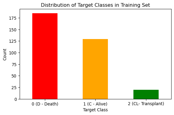
Make Numpy arrays for target sets
y_train = y_train_df.to_numpy()
y_test = y_test_df.to_numpy()
Models
Three supervised learning models are created to predict the status classes. For each type of model, two models are created: the first for the original imbalanced training set and the second for a resampled training set designed to address the class imbalance in the dataset.
Model validation and over-/under-fitting assessment
To validate each model and assess whether it is over- or under-fitting, a five-fold cross-validation was used, and the output from the cross-validation was used to plot the learning curves.
Cross-validation was chosen for the following reasons:
- Improves model performance estimation by using multiple data splits.
- Helps detect over-fitting by testing on varied subsets of data.
- Maximises use of limited data for both training and testing.
- Enables fair model comparison under consistent evaluation conditions.
Learning curves were used to interpret model performance because they:
- Can be used to diagnose under-fitting or over-fitting by comparing training and validation performance.
- Can guide model selection by comparing learning curves of different models to choose the best one.
The learning curve figures in this report show:
- F1 Macro Score (y-axis) versus the training set size (x-axis).
- Training score (red curve).
- Cross-validation score (green curve)
- Variability across folds (standard deviation) is shaded.
def run_cross_validate(model, X_train, y_train, label):
    """
    Function to perform cross-validation and plot learning curves

    :param model: Model to validate.
    :param X_train: Training data.
    :param y_train: TRaining labels.
    :returns: None
    """
    # Define stratified k-fold cross-validation
    cv = StratifiedKFold(n_splits=5)

    # Generate learning curve data
    train_sizes, train_scores, test_scores = learning_curve(
        model, X_train, y_train, cv=cv, scoring="f1_macro",
        train_sizes=np.linspace(0.1, 1.0, 10), n_jobs=-1
    )

    # Calculate mean and standard deviation
    train_scores_mean = np.mean(train_scores, axis=1)
    test_scores_mean = np.mean(test_scores, axis=1)
    train_scores_std = np.std(train_scores, axis=1)
    test_scores_std = np.std(test_scores, axis=1)

    # Plot the learning curve
    plt.figure(figsize=(10, 6))
    plt.title(f"Learning Curve for {label}")
    plt.xlabel("Training Set Size")
    plt.ylabel("F1 Macro Score")
    plt.grid(True)

    # Plot with shaded standard deviation
    plt.fill_between(train_sizes, train_scores_mean - train_scores_std,
                     train_scores_mean + train_scores_std, alpha=0.1, color="r")
    plt.fill_between(train_sizes, test_scores_mean - test_scores_std,
                     test_scores_mean + test_scores_std, alpha=0.1, color="g")

    plt.plot(train_sizes, train_scores_mean, 'o-', color="r", label="Training score")
    plt.plot(train_sizes, test_scores_mean, 'o-', color="g", label="Cross-validation score")

    plt.legend(loc="best")
    plt.tight_layout()

    # Save the figure
    plt.savefig(f"images/{label}_learning_curve.png")
Dealing with imbalance
To address the class imbalance, the Synthetic Minority Over-sampling Technique (SMOTE) was utilised to create a resampled training set. SMOTE generates synthetic samples for minority classes by interpolating between existing samples. SMOTE preserves all original data and avoids over-fitting.
# Apply SMOTE to balance all classes to match the majority class (class 0)
smote = SMOTE(random_state=0)
X_train_smote, y_train_smote = smote.fit_resample(X_train, y_train)

# Check new class distribution
smote_counts = pd.DataFrame(y_train_smote).value_counts()

# Plot the distribution
plt.figure(figsize=(6, 4))
smote_counts.plot(kind="bar", color=["red", "orange", "green"])
plt.title("Distribution of Target Classes in Resampled Training Set")
plt.xlabel("Target Class")
plt.ylabel("Count")
plt.xticks(ticks=[0, 1, 2], labels=["0 (D - Death)", "1 (C - Alive)", "2 (CL- Transplant)" ], rotation=0)
plt.tight_layout()
# Save the figure
plt.savefig("images/resampled_class_balance.png")
plt.show()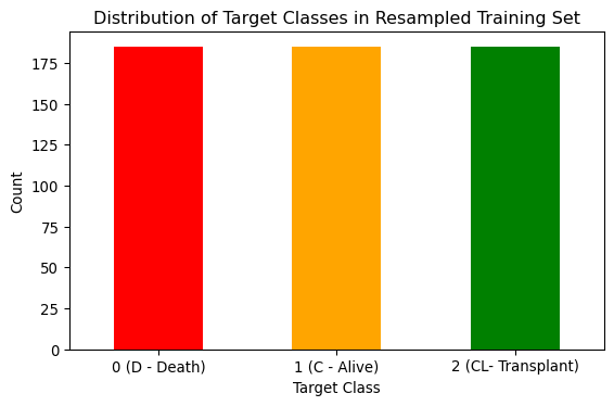
Model 1 - Logistic regression
Logistic regression was chosen as one of the models because it is simple and interpretable.
The logistic regression model in scikit-learn has several hyperparameters. Hyperparameter optimisation was performed to find the combination of parameters that gives the best model performance.
The Logistic regression hyperparameters are:
- Penalty: The regularisation method.
- C: The regularisation strength. Higher values give less regularisation.
- Solver: The type of solver used.
- Maximum Iterations: Controls how long the solver runs.
- Tolerance: Determines the stopping criteria for the optimisation.
- Class Weight: Useful for imbalanced datasets.
As this is a multi-class problem, the only solver that can handle such problems and supports none, L1 and L2 regularisation is “saga”. Therefore, the solver type was removed from the hyperparameter tuning.
The scikit-learn GridSearchCV is used to execute the parameter tuning. It runs through all combinations of the parameters and uses cross-validation to evaluate the model’s performance. The macro version of the F1 score was used for the model evaluation during the grid search. F1 is the harmonic mean of precision and recall. The macro option calculates metrics for each class and finds their unweighted mean. The main objective of this work is to predict the “Status” of patients accurately. Therefore, the aim is to strike a balance between the recall and the precision. The number of folds in the cross-validation was chosen to be five to balance performance with confidence. More folds will give higher confidence in the result; However, this comes at an additional computational cost.
def run_grid_search_lr(X_train, y_train):
    """
    Function to run a grid search for hyperparameter tuning of logistic regression models.

    :param X_train: Feature training set
    :param y_train: Label training set
    :returns: GridSearchCV model
    """
    # Initialise model
    logreg_model = LogisticRegression(solver="saga", random_state=0)

    # Create parameter grid
    param_grid = {
        "penalty": [None, "l1", "l2"],
        "C": [0.0001, 0.001, 0.01, 0.1, 1.0, 10.0, 100.0],
        "class_weight": [None, "balanced"],
        "max_iter": [100, 500, 1000],
        "tol": [1e-5, 1e-4, 1e-3],
    }

    # Set up GridSearchCV
    # GridSearchCV uses stratified sampling internally, so no special action is required.
    # Interested in performance for all classes, so use the macro option
    grid_search = GridSearchCV(logreg_model, param_grid, cv=5, scoring="f1_macro", n_jobs=-1,
                               return_train_score=True)

    # Fit the model
    grid_search.fit(X_train, y_train)

    # Convert results to DataFrame
    results_df = pd.DataFrame(grid_search.cv_results_)

    # Create a readable label for each parameter combination
    results_df["param_combo"] = results_df.apply(
        lambda row: f"{row['param_penalty']}, C={row['param_C']}, iter={row['param_max_iter']}, tol={row['param_tol']}, weight={row['param_class_weight']}",
        axis=1
    )

    top_10 = results_df.sort_values(by="mean_test_score", ascending=False).head(10)
    print("Top 10 parameters combinations results")
    print(top_10[["param_combo", "mean_test_score"]].to_string(index=False))

    # Best parameters and score
    print("\nBest Parameters:", grid_search.best_params_)
    print(f"Best Score: {grid_search.best_score_:.4f}")

    return grid_search
Logistic regression hyperparameter tuning with original data
# Run GridSearch on original data
grid_original = run_grid_search_lr(X_train, y_train)
Top 10 parameters combinations results
param_combo mean_test_score
l2, C=0.1, iter=500, tol=0.0001, weight=balanced 0.574750
l2, C=0.1, iter=100, tol=1e-05, weight=balanced 0.574750
l2, C=0.1, iter=100, tol=0.0001, weight=balanced 0.574750
l2, C=0.1, iter=1000, tol=1e-05, weight=balanced 0.574750
l2, C=0.1, iter=1000, tol=0.0001, weight=balanced 0.574750
l2, C=0.1, iter=500, tol=1e-05, weight=balanced 0.574750
l2, C=0.1, iter=1000, tol=0.001, weight=balanced 0.574049
l2, C=0.1, iter=500, tol=0.001, weight=balanced 0.574049
l2, C=0.1, iter=100, tol=0.001, weight=balanced 0.574049
l2, C=0.01, iter=100, tol=0.0001, weight=balanced 0.555429
Best Parameters: {'C': 0.1, 'class_weight': 'balanced', 'max_iter': 100, 'penalty': 'l2', 'tol': 1e-05}
Best Score: 0.5748Train the model using the best parameters
logreg_bm = grid_original.best_estimator_
logreg_bm.fit(X_train, y_train)
LogisticRegression(C=0.1, class_weight='balanced', random_state=0,
solver='saga', tol=1e-05)In a Jupyter environment, please rerun this cell to show the HTML representation or trust the notebook. On GitHub, the HTML representation is unable to render, please try loading this page with nbviewer.org.
Parameters
| penalty | 'l2' | |
| dual | False | |
| tol | 1e-05 | |
| C | 0.1 | |
| fit_intercept | True | |
| intercept_scaling | 1 | |
| class_weight | 'balanced' | |
| random_state | 0 | |
| solver | 'saga' | |
| max_iter | 100 | |
| multi_class | 'deprecated' | |
| verbose | 0 | |
| warm_start | False | |
| n_jobs | None | |
| l1_ratio | None |
run_cross_validate(logreg_bm, X_train, y_train, "Logistic Regression (original data)")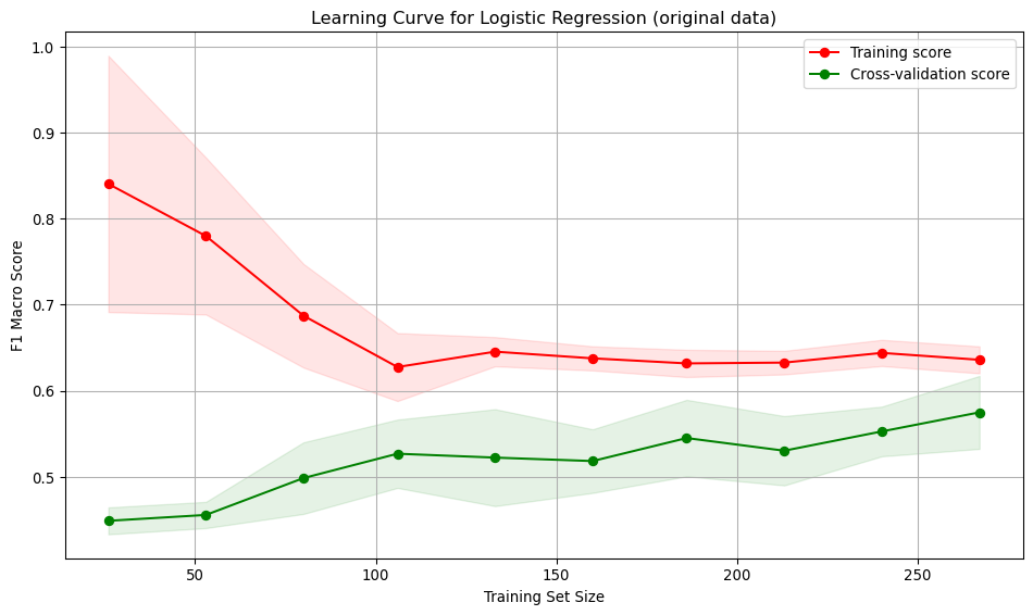
Interpretation:
- As the model sees more data, it becomes less tailored to the small initial training set and generalises more, resulting in a drop in the training score. The drop suggests the model is no longer over-fitting to small samples.
- The cross-validation score increases, then stabilises as training size grows beyond 100. The model is learning and generalising better.
- The training and test curves become parallel, suggesting the model is not over-fitting.
- The low value for the score for both the training and validation curves indicates the model is under-fitting.
- The variation across folds suggests the model’s performance across folds is consistent, indicating stability and reliability.
Logistic model - SMOTE resampled data
Since the resampled training dataset is different, there is no guarantee that the previously identified hyperparameters will still be optimal for this dataset. Therefore, the grid search was repeated to find the combination of parameters that gave the best performance for the resampled training data.
# Run GridSearch on SMOTE-balanced data
grid_smote = run_grid_search_lr(X_train_smote, y_train_smote)
logreg_bm_smote = grid_smote.best_estimator_

run_cross_validate(logreg_bm_smote, X_train_smote, y_train_smote, "Logistic Regression (SMOTE resampled data)")
Top 10 parameters combinations results
param_combo mean_test_score
l2, C=0.1, iter=500, tol=0.001, weight=balanced 0.704506
l2, C=0.1, iter=1000, tol=0.001, weight=balanced 0.704506
l2, C=0.1, iter=100, tol=0.001, weight=None 0.704506
l2, C=0.1, iter=500, tol=0.001, weight=None 0.704506
l2, C=0.1, iter=1000, tol=0.001, weight=None 0.704506
l2, C=0.1, iter=100, tol=0.001, weight=balanced 0.704506
l2, C=0.1, iter=500, tol=0.0001, weight=balanced 0.702595
l2, C=0.1, iter=1000, tol=1e-05, weight=balanced 0.702595
l2, C=0.1, iter=1000, tol=0.0001, weight=balanced 0.702595
l2, C=0.1, iter=500, tol=1e-05, weight=balanced 0.702595
Best Parameters: {'C': 0.1, 'class_weight': None, 'max_iter': 100, 'penalty': 'l2', 'tol': 0.001}
Best Score: 0.7045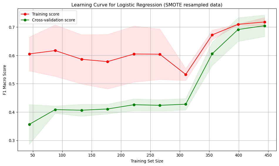
Interpretation: * Training score starts high (~0.6) and remains relatively stable, ending around ~0.7. Indicates the model fits the training data well, even with small datasets. * Cross-validation score starts low (~0.35) and steadily improves with more training data, reaching ~0.72. Suggests the model generalises better as it sees more data. * Large gap between training curves at small training sizes, implying overfitting. The model performs well on training data but poorly on unseen data. * The gap narrows with more data, indicating improved generalisation and reduced overfitting. * At low sample numbers, the variance across folds is high. This narrows as more training data is added.
# Report results
print("Original Data Performance:")
print("Best Parameters:", grid_original.best_params_)
print("\nSMOTE-Balanced Data Performance:")
print("Best Parameters:", grid_smote.best_params_)
Original Data Performance:
Best Parameters: {'C': 0.1, 'class_weight': 'balanced', 'max_iter': 100, 'penalty': 'l2', 'tol': 1e-05}
SMOTE-Balanced Data Performance:
Best Parameters: {'C': 0.1, 'class_weight': None, 'max_iter': 100, 'penalty': 'l2', 'tol': 0.001}Model 2 - SVC
SVC was chosen as one of the models because it is effective in high-dimensional spaces and works well with small datasets.
The SVC model in scikit-learn has several hyperparameters, and hyperparameter optimisation was performed to find the combination of parameters that gives the best model performance.
The SVC hyperparameters are:
- Kernel: Options are “linear”, “RBF”, “poly” and “sigmoid”.
- C: Regularisation parameter. Controls the trade-off between accuracy and generalisation. Available for all kernels.
- High values create tighter decision boundaries (risk of overfitting).
- Low values allow smoother decision boundaries (risk of underfitting).
- High values create tighter decision boundaries (risk of overfitting).
- Class Weight: Useful for imbalanced datasets.
Kernel-specific hyperparameters:
- “gamma”: Influence of individual data points. Available in “RBF”, “poly”, and “sigmoid”.
- Higher values make the model focus on local structures (risk of overfitting).
- Lower values create smoother decision boundaries.
- “coef0”: Controls curve shift in polynomial/sigmoid kernels.
- Impacts feature interactions.
- “degree”: Defines the complexity of polynomial curves.
- Higher degrees create more flexible decision boundaries.
As there are a large number of possible combinations of hyperparameters. BayesSearchCV was used to explore the hyperparameter search space, as it is more efficient than a brute-force grid search. Again, a five-fold cross-validation with the macro version of the F1 score is used for model evaluation during the search.
def run_search_svm(X_train, y_train):
    """
    Function to run a Bayes search for hyperparameter tuning of SVM models.

    :param X_train: Feature training set
    :param y_train: Label training set
    :returns: BayesSearchCV model
    """
    search_space = {
        "kernel": ["linear", "rbf", "poly", "sigmoid"],
        "C": (1e-3, 1e3, 'log-uniform'),
        "class_weight": [None, "balanced"],
        "gamma": (1e-4, 1, 'log-uniform'),
        "degree": (2, 5),
        "coef0": (-1, 1)
    }

    opt = BayesSearchCV(
        SVC(probability=False, max_iter = -1, tol = 1e-3, verbose=True, random_state=0),
        search_spaces=search_space,
        scoring="f1_macro",
        cv=StratifiedKFold(n_splits=5),
        n_iter=50,  # Number of iterations
        n_jobs=-1,  # Use all cores
        verbose=0,
        random_state=0
    )

    opt.fit(X_train, y_train)

    # Convert results to DataFrame
    results_df = pd.DataFrame(opt.cv_results_)

    # Create a readable label for each parameter combination
    results_df["param_combo"] = results_df.apply(
        lambda row: f"{row['param_kernel']}, C={row['param_C']:.4f}, "
                    f"weight={row['param_class_weight']}, gamma={row['param_gamma']:.4f},"
                    f"degree={row['param_degree']}, coef0={row['param_coef0']},",
        axis=1
    )

    top_10 = results_df.sort_values(by="mean_test_score", ascending=False).head(10)
    print("\nTop 10 parameters combinations results")
    print(top_10[["param_combo", "mean_test_score"]].to_string(index=False))

    print("Best parameters:", opt.best_params_)
    print("Best score:", opt.best_score_)

    return opt
SVC hyperparameter tuning with original data
# Run GridSearch on original data
grid_original_svm = run_search_svm(X_train, y_train)
[LibSVM]
Top 10 parameters combinations results
param_combo mean_test_score
linear, C=0.0407, weight=balanced, gamma=0.0005,degree=4, coef0=0, 0.578629
linear, C=0.0395, weight=balanced, gamma=0.0001,degree=3, coef0=-1, 0.575117
linear, C=0.0387, weight=balanced, gamma=0.0001,degree=2, coef0=-1, 0.575117
linear, C=0.0368, weight=balanced, gamma=0.0001,degree=2, coef0=0, 0.574452
linear, C=0.0563, weight=balanced, gamma=0.0004,degree=2, coef0=-1, 0.572485
linear, C=0.0355, weight=balanced, gamma=0.0011,degree=4, coef0=1, 0.571958
linear, C=0.0224, weight=balanced, gamma=0.0004,degree=4, coef0=-1, 0.567018
linear, C=0.0701, weight=balanced, gamma=0.0010,degree=4, coef0=-1, 0.562934
linear, C=0.0797, weight=balanced, gamma=0.0002,degree=5, coef0=0, 0.562934
sigmoid, C=392.2376, weight=balanced, gamma=0.0001,degree=2, coef0=-1, 0.553314
Best parameters: OrderedDict([('C', 0.04069971836887072), ('class_weight', 'balanced'), ('coef0', 0), ('degree', 4), ('gamma', 0.00047722740319078804), ('kernel', 'linear')])
Best score: 0.5786290642921209svm_bm = grid_original_svm.best_estimator_
svm_bm.fit(X_train, y_train)[LibSVM]SVC(C=0.04069971836887072, class_weight='balanced', coef0=0, degree=4,
gamma=0.00047722740319078804, kernel='linear', random_state=0,
verbose=True)In a Jupyter environment, please rerun this cell to show the HTML representation or trust the notebook. On GitHub, the HTML representation is unable to render, please try loading this page with nbviewer.org.
Parameters
| C | 0.04069971836887072 | |
| kernel | 'linear' | |
| degree | 4 | |
| gamma | 0.00047722740319078804 | |
| coef0 | 0 | |
| shrinking | True | |
| probability | False | |
| tol | 0.001 | |
| cache_size | 200 | |
| class_weight | 'balanced' | |
| verbose | True | |
| max_iter | -1 | |
| decision_function_shape | 'ovr' | |
| break_ties | False | |
| random_state | 0 |
Model validation and over-/under-fitting assessment
run_cross_validate(svm_bm, X_train, y_train, "SVC (original data)")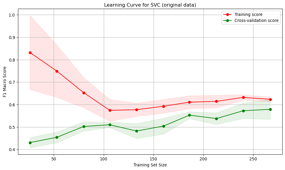
Interpretation:
- Training score starts high (~0.82) with small data, then decreases and stabilises around 0.61. Indicates the model initially over-fits but generalises better with more data.
- Cross-validation score starts low (~0.42) and steadily improves with more training data, reaching ~0.58. Suggests the model generalises better as it sees more data.
- Large gap between training curves at small training sizes, implying over-fitting. The model performs well on training data but poorly on unseen data.
- The gap narrows with more data, indicating improved generalisation and reduced over-fitting.
- The low value for the score for both the training and validation curves indicates the model is under-fitting.
- At low sample numbers, the variance across folds is high, narrowing as more training data is added.
SVC model - SMOTE resampled data
# Run GridSearch on SMOTE-balanced data
grid_svm_smote = run_search_svm(X_train_smote, y_train_smote)
svm_bm_smote = grid_svm_smote.best_estimator_

run_cross_validate(svm_bm_smote, X_train_smote, y_train_smote, "SVC (SMOTE resampled data)")
[LibSVM]
Top 10 parameters combinations results
param_combo mean_test_score
rbf, C=1000.0000, weight=None, gamma=0.0178,degree=5, coef0=1, 0.820066
rbf, C=1000.0000, weight=None, gamma=0.1240,degree=5, coef0=1, 0.818908
rbf, C=458.5276, weight=balanced, gamma=0.0258,degree=5, coef0=-1, 0.811727
rbf, C=1000.0000, weight=balanced, gamma=0.0223,degree=5, coef0=1, 0.808890
rbf, C=1000.0000, weight=None, gamma=0.0220,degree=5, coef0=-1, 0.806786
rbf, C=1000.0000, weight=None, gamma=0.0046,degree=5, coef0=1, 0.800797
rbf, C=1000.0000, weight=balanced, gamma=0.0445,degree=2, coef0=1, 0.800797
rbf, C=1000.0000, weight=None, gamma=0.0257,degree=5, coef0=1, 0.799462
poly, C=1000.0000, weight=balanced, gamma=0.0498,degree=5, coef0=1, 0.791560
rbf, C=1000.0000, weight=None, gamma=0.0295,degree=5, coef0=1, 0.790761
Best parameters: OrderedDict([('C', 1000.0), ('class_weight', None), ('coef0', 1), ('degree', 5), ('gamma', 0.017811344333727035), ('kernel', 'rbf')])
Best score: 0.8200656061445114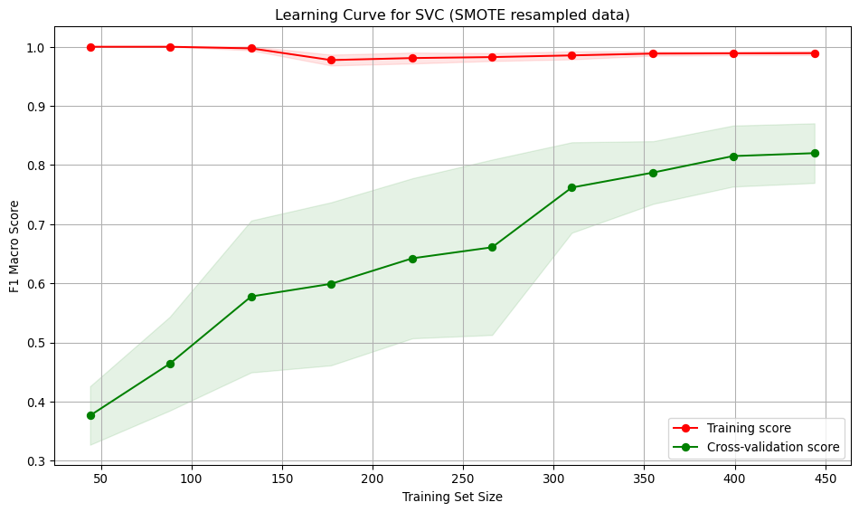
Interpretation:
- Training score starts at 1.0, dips slightly and then ends near 1.0. The model is over-fitting the training data. Possibly due to the high C value.
- Cross-validation score starts low (~0.38) and steadily improves with more training data, reaching ~0.82. Suggests the model generalises better as it sees more data.
- Large gap between training curves at small training sizes, implying over-fitting. The model performs well on training data but poorly on unseen data.
- The gap narrows with more data, indicating improved generalisation and reduced over-fitting.
- At low sample numbers, the variance across folds is high, narrowing as more training data is added.
Model 3 - Decision Tree
A decision tree was chosen as one of the models because it is interpretable and handles non-linear relationships. The Decision Tree classifier in scikit-learn has many hyperparameters, mainly focused on early stopping of tree growth (pre-pruning). Whilst a Bayes or grid search could be used to find the optimal values for each of these hyperparameters, those approaches still require selecting an appropriate search space. An alternative approach to pre-pruning (pruning during growth) is post-pruning. In post-pruning, a full tree is grown and then pruned to remove branches that do not improve the performance. This approach is well-suited to small datasets, such as in this study and is the approach used.
Training an unpruned tree
# Train an unpruned decision tree
unpruned_tree = DecisionTreeClassifier(random_state=0)
unpruned_tree.fit(X_train, y_train)

# Plot the decision tree
plt.figure(figsize=(12, 8))
plot_tree(unpruned_tree, filled=True, feature_names=X_train_enc_df.columns, class_names=["D", "C", "CL" ])
plt.title("Decision Tree Trained on original dataset")
plt.savefig("images/full_tree.png")
plt.show()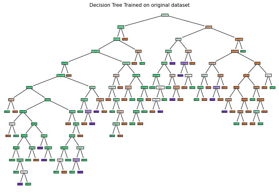
run_cross_validate(unpruned_tree, X_train, y_train, "Decision Tree (unpruned original data)")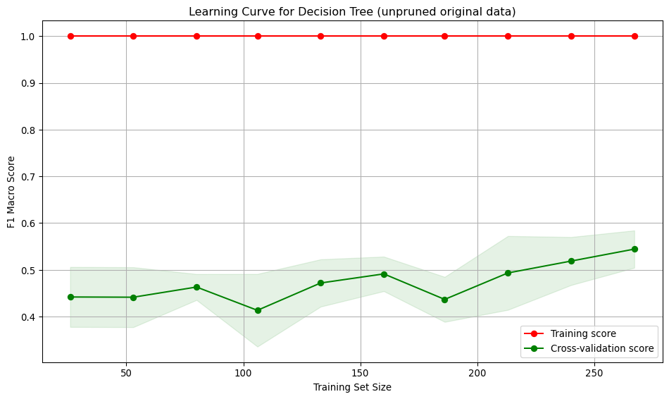
Tree pruning
Here, the unpruned tree is used to obtain the cost-complexity path values. Then, using the cost complexity values, many trees are built, each with a different cost complexity value. A 5-fold stratified cross-validation is used to assess the macro F1 score for each of the pruned trees. The pruned tree that gives the highest mean cross-validation macro F1 score is chosen as the best tree.
def tree_pruning(full_tree, X_train, y_train, label):

    # Get cost-complexity pruning path
    path = full_tree.cost_complexity_pruning_path(X_train, y_train)
    ccp_alphas = path.ccp_alphas

    # Train trees with different ccp_alpha values (no pre-pruning settings)
    trees = []
    for alpha in ccp_alphas:
        clf = DecisionTreeClassifier(random_state=0, ccp_alpha=alpha)
        clf.fit(X_train, y_train)
        trees.append(clf)

    # Define stratified k-fold cross-validation
    cv = StratifiedKFold(n_splits=5)

    # Evaluate each tree using cross-validation
    cv_scores = []
    for clf in trees:
        scores = cross_val_score(clf, X_train, y_train, cv=cv, scoring="f1_macro")
        cv_scores.append(np.mean(scores))

    # Find the best pruned tree
    best_index = np.argmax(cv_scores)
    best_pruned_tree = trees[best_index]
    best_alpha = ccp_alphas[best_index]
    best_score = cv_scores[best_index]

    # Print the best alpha and corresponding score
    print(f"Best ccp_alpha: {best_alpha:.4f}")
    print(f"Best cross-validation accuracy: {best_score:.4f}")

    # Plot accuracy vs ccp_alpha
    plt.figure(figsize=(10, 6))
    plt.plot(ccp_alphas, cv_scores, marker='o', drawstyle="steps-post")
    plt.xlabel("ccp_alpha")
    plt.ylabel("Macro F1-score")
    plt.title(f"F1-score vs CCP Alpha for Pruned Decision Trees {label}")
    plt.grid(True)
    plt.tight_layout()
    plt.savefig(f"images/pruning_accuracy_comparison{label}.png")

    return best_pruned_tree
best_pruned_tree = tree_pruning(unpruned_tree, X_train, y_train, label="(original data)")Best ccp_alpha: 0.0095
Best cross-validation accuracy: 0.6100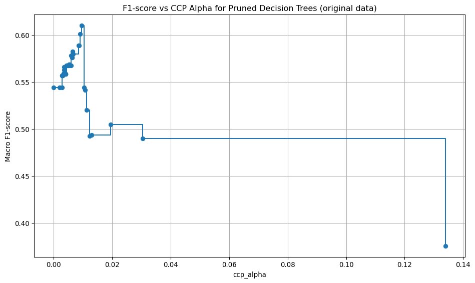
Model evaluation: original data, best pruning
run_cross_validate(best_pruned_tree, X_train, y_train, "Decision Tree (best pruned, original data)")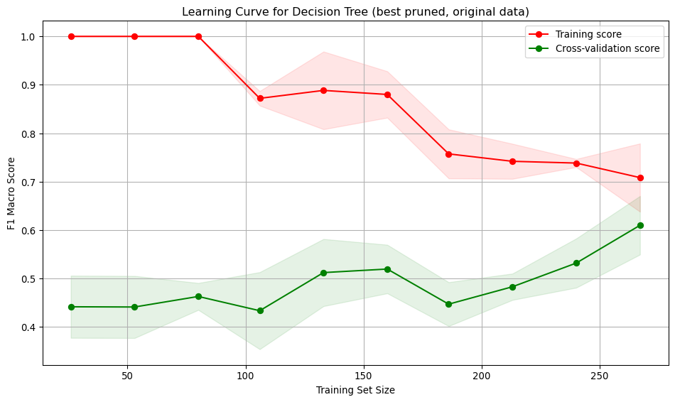
Interpretation:
- Training score starts at 1, indicating over-fitting on small datasets. As the training set size increases, the score drops and stabilises around 0.7, showing the model generalises better for larger training set sizes.
- Cross-validation score starts low (~0.45) and gradually increases reaching ~0.6. Suggests the model generalises better as it sees more data, but performance is low.
- Large gap between training curves at small training sizes, implying over-fitting. The model performs well on training data but poorly on unseen data. The gap narrows with more data, indicating improved generalisation and reduced over-fitting.
- At low sample numbers, the variance across folds is low for the training and moderate for the validation. As more training data is added, the variation across folds increases for the training set and decreases slightly for the validation.
# Plot the best decision tree
plt.figure(figsize=(12, 8))
plot_tree(best_pruned_tree, filled=True, feature_names=X_train_enc_df.columns, class_names=["D", "C", "CL" ])
plt.title("Best Pruned Decision Tree Trained on original dataset")
plt.savefig("best_decision_tree_origdata.png")
plt.show()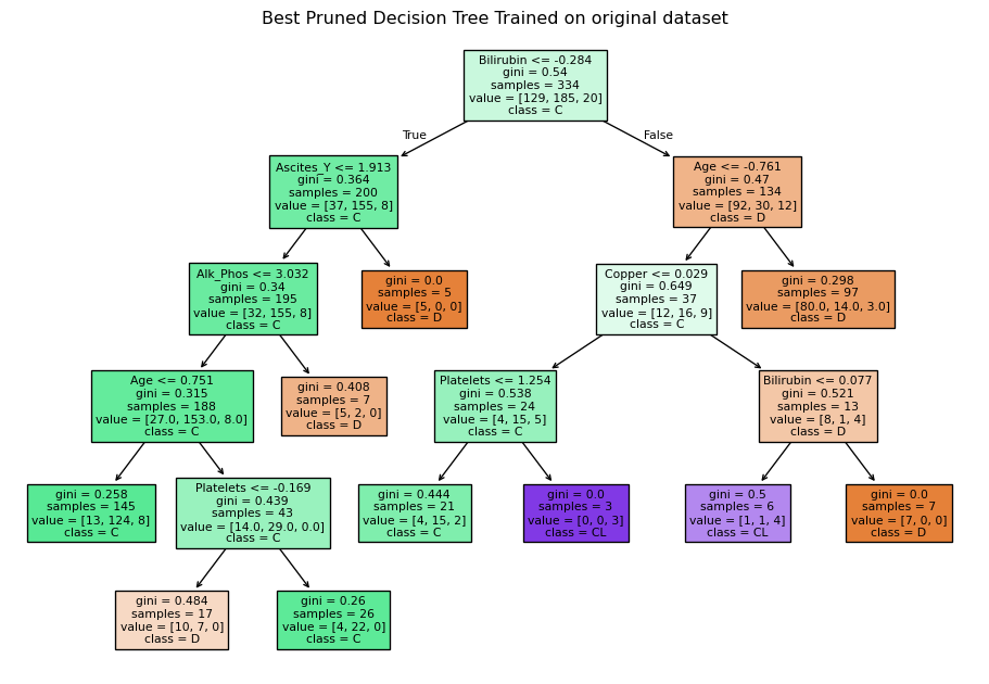
Training an unpruned tree using resampled data
# Train an unpruned decision tree
unpruned_tree_sm = DecisionTreeClassifier(random_state=0)
unpruned_tree_sm.fit(X_train_smote, y_train_smote)

# Plot the decision tree
plt.figure(figsize=(12, 8))
plot_tree(unpruned_tree_sm, filled=True, feature_names=X_train_enc_df.columns, class_names=["D", "C", "CL" ])
plt.title("Decision Tree Trained on resampled dataset")
plt.savefig("images/full_tree_smote.png")
plt.show()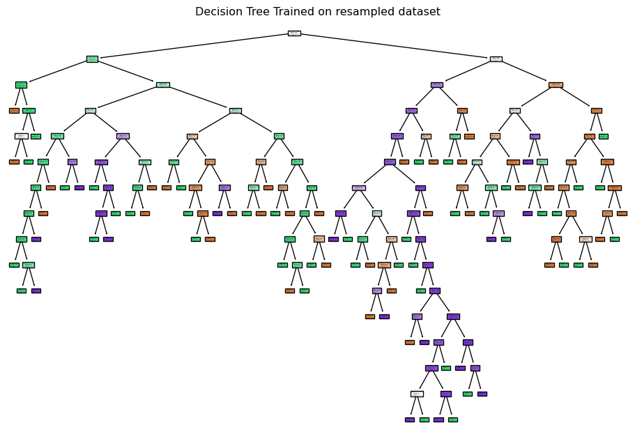
Tree pruning: resampled data
best_pruned_tree_smote = tree_pruning(unpruned_tree_sm, X_train_smote, y_train_smote, label="(resampled data)")Best ccp_alpha: 0.0056
Best cross-validation accuracy: 0.7422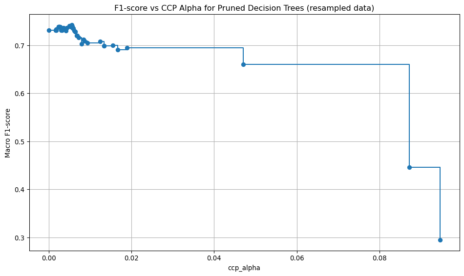
Model evaluation: resampled data, best pruning
run_cross_validate(best_pruned_tree_smote, X_train_smote, y_train_smote, "Decision Tree (best pruned, resampled data)")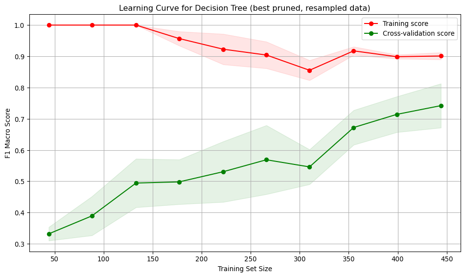
Interpretation: * Training score starts at 1, indicating over-fitting on small datasets. As the training set size increases, the score drops slightly but remains high, indicating the model continues to fit the training data well. * Cross-validation score starts low (~0.33) and gradually increases reaching ~0.75. Suggests the model generalises better as it sees more data, and the performance is higher. * Large gap between training curves at small training sizes, implying over-fitting. The model performs well on training data but poorly on unseen data. The gap narrows with more data, indicating improved generalisation and reduced over-fitting.
* The training curve shows low variation across folds. The validation curve shows moderate variation, especially at smaller training sizes. This variation decreases as the training size increases, indicating a more stable performance on unseen data.
# Plot the best decision tree
plt.figure(figsize=(12, 8))
plot_tree(best_pruned_tree_smote, filled=True, feature_names=X_train_enc_df.columns, class_names=["D", "C", "CL" ])
plt.title("Best Pruned Decision Tree Trained on resampled dataset")
plt.savefig("best_decision_tree_resampleddata.png")
plt.show()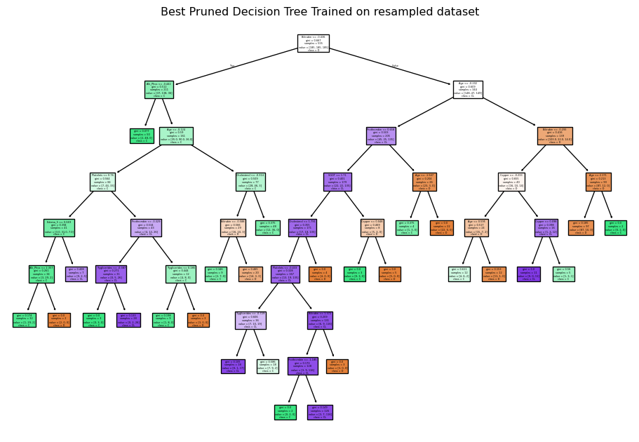
Recommended model
According to the reported results above, all three models using the original training data exhibited under-fitting. Using the resampled data, the SVC model showed signs of over-fitting. Both the logistic regression and decision tree models demonstrate a balance between over- and under-fitting. While the decision tree model shows a higher macro F1 score (0.7422) compared to the logistic regression (0.7045), the logistic regression model has a much lower variation in the validation score, indicating it is more stable across folds and the gap between the training and validation error was smallest. Therefore, the logistic regression model trained on the resampled data is recommended.
Prediction
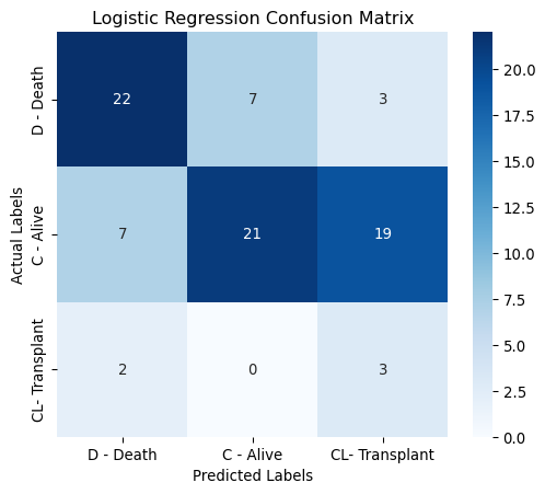
The figure below displays the confusion matrix for the recommended logistic regression model evaluated using the test set. The model performs reasonably well in predicting deaths (D) and alive (C) cases. It struggles most with transplant (CL) cases, especially confusing them with alive (C).
Correct Predictions - 22 deaths correctly predicted as deaths. - 22 alive correctly predicted as alive. - 3 transplants were correctly predicted as transplants.
Misclassifications - 7 deaths predicted as alive, 3 as transplant. - 8 alive predicted as death, 17 as transplant. - 2 transplants predicted as death.
# Predict on test set
y_pred = logreg_bm_smote.predict(X_test)

print(classification_report(y_test, y_pred, target_names=["D", "C", "CL"], digits=4))

# Plot Confusion Matrix
classes = ["D - Death", "C - Alive", "CL- Transplant" ]
cm = confusion_matrix(y_test, y_pred, labels=[0,1,2])
plt.figure(figsize=(6, 5))
sns.heatmap(cm, annot=True, fmt="d", cmap="Blues", xticklabels=classes, yticklabels=classes)
plt.xlabel("Predicted Labels")
plt.ylabel("Actual Labels")
plt.title(f"Logistic Regression Confusion Matrix")
plt.savefig("images/lr_confusion.png")
plt.show()
precision recall f1-score support
D 0.7097 0.6875 0.6984 32
C 0.7500 0.4468 0.5600 47
CL 0.1200 0.6000 0.2000 5
accuracy 0.5476 84
macro avg 0.5266 0.5781 0.4861 84
weighted avg 0.6971 0.5476 0.5913 84
Feature importance
Two methods were used to analyse feature importance:
- Permutation importance - evaluates how much a model’s performance decreases when a feature’s values are randomly shuffled. If shuffling a feature significantly worsens the model’s performance, that feature is considered important.
- SHAP analysis - ensures robust statistical inference by examining feature contributions at both individual and aggregate levels, while accounting for potential non-linear effects and class-specific patterns in the data.
# Permutation importance
result = permutation_importance(logreg_bm_smote, X_test, y_test, n_repeats=100, random_state=0, scoring="f1_macro")

# Create DataFrame for visualization
importance_df = pd.DataFrame({
    "Feature": X_train_enc_df.columns,
    "Importance Mean": result.importances_mean,
    "Importance Std": result.importances_std
}).sort_values(by="Importance Mean", ascending=True)

# Plot permutation importance
plt.figure(figsize=(10, 8))
plt.barh(importance_df["Feature"], importance_df["Importance Mean"], xerr=importance_df["Importance Std"])
plt.xlabel("Mean Importance")
plt.title("Permutation Feature Importance")
plt.tight_layout()
plt.savefig("images/permutation_importance.png")
plt.show()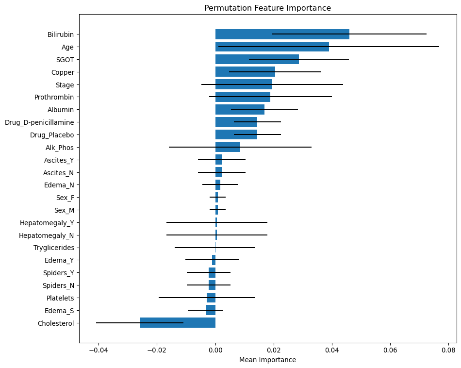
The bar length shows the mean importance values. Positive values indicate that these features contribute positively to the model’s predictive power. Negative values suggest that shuffling the feature actually improved model performance, implying it may be noise or negatively correlated with the target. The error bars represent the standard deviation from multiple permutations. Wide error bars crossing zero imply low confidence in the feature’s importance.
Permutation importance summary
Most Important features
- Bilirubin and Age are the most statistically significant predictors — high mean importance.
Moderate Important features
- SGOT, Copper, Stage, Prothrombin, Albumin, and Drug are also moderate predictors.
Less important
- Ascite, Edema_N, Sex, Hepatomegaly and Tryglicerides are not important.
- Edema_Y/S, Spiders, Platelets and Cholesterol may be redundant - negative importance.
explainer = shap.Explainer(logreg_bm_smote, X_test)
shap_values = explainer(X_test)

# Summary plot
plt.figure()
shap.summary_plot(shap_values, X_test, feature_names= X_train_enc_df.columns, max_display=24, show=False)
plt.savefig("images/shap_summary_plot.png")
plt.show()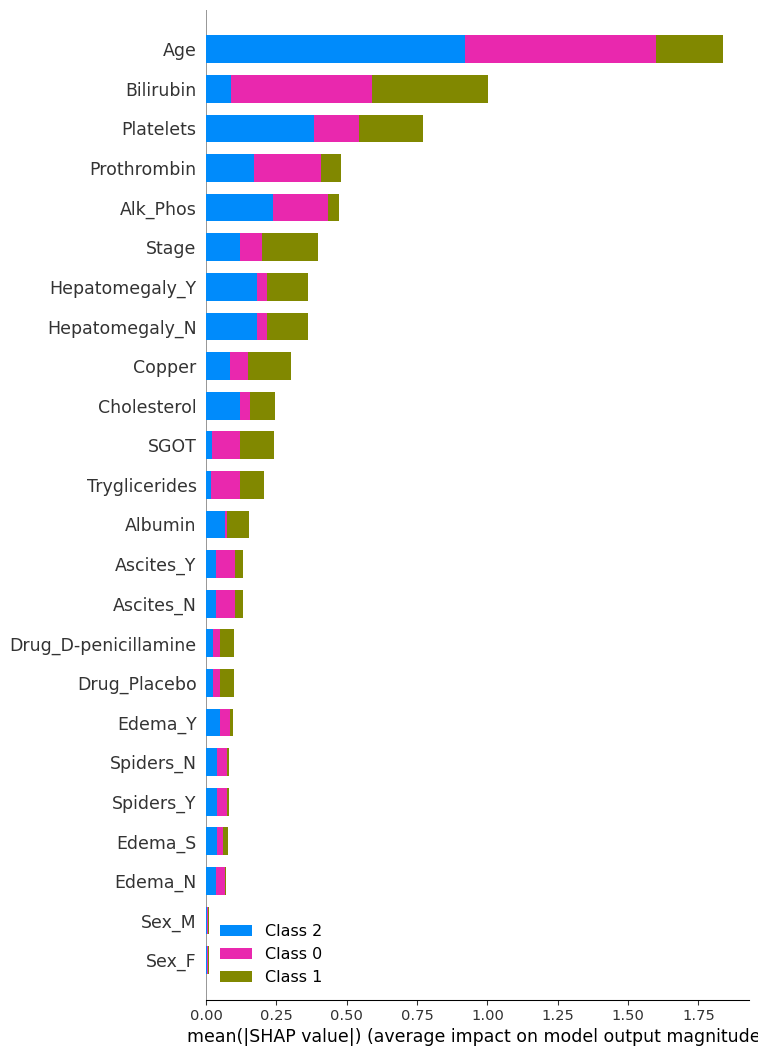
The bar length represents the average magnitude of the SHAP values for each feature across all samples. A higher value means the feature has a greater impact on the model’s predictions. Each colour corresponds to a class in the classification problem, showing how each feature contributes to different classes.
SHAP analysis summary
Most Important features
- Age, Bilirubin: Their high SHAP values suggest they consistently influence the model’s output across samples.
Moderate Important features
- Platelets, Prothrombin, Alk_Phos, Stage, Hepatomegaly, and Copper: Their moderate SHAP values suggest they consistently influence the model’s output across samples.
Less important
- Sex, Edema, Spiders and Drug. Their low SHAP values suggest they consistently do not influence the model’s output across samples.
Class-Specific Contributions:
- Age is most influential in predicting Class 2 and 0.
- Bilirubin is the most influential in predicting Classes 1.
SHAP vs. Permutation Importance
Most Important Features (Both Methods Agree)
- Bilirubin: Top-ranked in both SHAP and permutation importance — strong indicator of liver function.
- Age: Highly ranked in both — likely reflects disease progression or risk stratification.
Moderately Important Features
- Albumin, Alk_Phos, SGOT, Stage, Prothrombin, Platelets: These appear in both plots with moderate importance, suggesting consistent influence across methods.
Least Important Features (Both Methods Agree)
- Sex, Edema, Spiders
Discrepancies
- Drug: More prominent in permutation importance than SHAP.
- Hepatomegaly: More prominent in SHAP than permutation importance.
- Cholesterol: Ranked lowest in permutation importance (even negative), but has some presence in SHAP — possibly due to interaction effects captured by SHAP but not permutation.