Linear programming and Game Theory

Q1

A food factory is making a beverage for a customer from mixing two different existing products A and B. The compositions of A and B and prices ($/L) are given as follows,

Juice Blend	Lime (L/100L)	Orange (L/100L)	Mango (L/100L)	Cost ($/L)
A	2	6	4	5
B	7	4	8	15

The customer requires that there must be at least 5 Litres (L) Orange and at least 5 Litres of Mango concentrate per 100 Litres of the beverage respectively, but no more than 6 Litres of Lime concentrate per 100 Litres of beverage. The customer needs at least 150 Litres of the beverage per week.

(a)

This problem requires a best outcome (minimising cost) where the requirements of the problem (objective and constraint functions) are represented by linear relationships of the decision variables.

(b)

Decision variables:

Let \(x_1\) be the number of litres of product A used per week and \(x_2\) be the number of litres of product B used each week.

Objective function:

Minimise the cost of production. Product A costs $5/L and product B $15/L.

\[ \text{Minimise Cost } = 5x_1 +15x_2 \]

Constraints:

The amount of lime must be \(\leq 0.06\)L/L. Product A provides 0.02 L of lime per L, and product B provides 0.07 L of lime per L.

\[ 0.02x_1+0.07x_2 \leq 0.06(x_1+x_2) \]

This can be rearranged to

\[ -0.04x_1+0.01x_2 \leq 0 \]

This can be simplified to

\[ -4x_1+x_2 \leq 0 \]

The amount of orange must be \(\geq 0.05\)L/L. Product A provides 0.06 L of orange per L, and product B provides 0.04 L of orange per L.

\[ 0.06x_1+0.04x_2 \geq 0.05(x_1+x_2) \]

This can be rearranged to

\[ 0.01x_1-0.01x_2 \geq 0 \]

This can be simplified to

\[ x_1-x_2 \geq 0 \]

The amount of mango must be \(\geq 0.05\)L/L. Product A provides 0.04 L of mango per L, and product B provides 0.08 L of mango per L.

\[ 0.04x_1+0.08x_2 \geq 0.05(x_1+x_2) \]

This can be rearranged to

\[ -0.01x_1+0.03x_2 \geq 0 \]

This can be simplified to

\[ -\frac{1}{3}x_1+x_2 \geq 0 \]

The total volume of weekly beverage required is \(\geq 150\) L.

\[ x+1+x_2 \geq 150 \]

LP model summary

Minimise \(z=5x_1 +15x_2\)

Subject to:

\[ \begin{align*} -4x_1+x_2 &\leq 0 \text{ (Lime constraint)} \\ x_1-x_2 &\geq 0 \text{ (Orange constraint)} \\ -\frac{1}{3}x_1+x_2 &\geq 0 \text{ (Mango constraint)} \\ x_1+x_2 &\geq 150 \text{ (Volume constraint)}\\ x_1 &\geq 0 \text{ (Non-negative constraint)} \\ x_2 &\geq 0 \text{ (Non-negative constraint)} \end{align*} \]

(c)

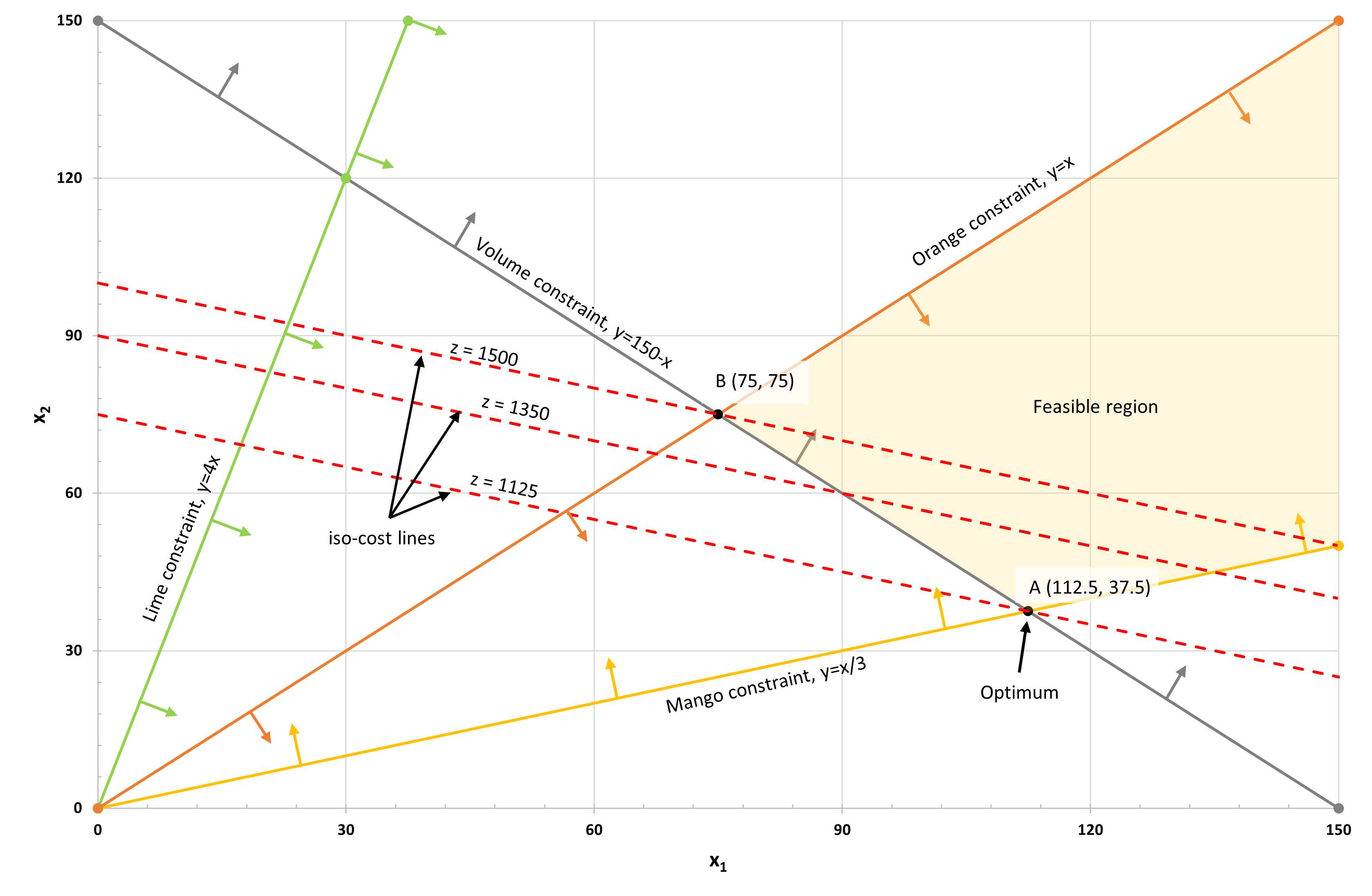
The optimum values of the decision variables to minimise the cost of production found using the graphical method are 112.5L of product A and 37.5L of product B.

Figure 1: Graphical solution for the linear programming problem, showing the feasible region and the optimum point A (112.5, 37.5).

(d)

The iso-cost line is

\[ x_2 = -\frac{1}{3}x_1 + \frac{\text{const}}{15} \]

A parameterised iso-cost line is

\[ x_2 = -\frac{c_1}{15}x_1 + \frac{\text{const}}{15} \]

We need to find the range of values for \(c_1\) where the current optimum (point A) would still be optimal. The slope of the volume and mango constraints bound the solution at point A. The volume constraint slope is \(=-1\), and the mango constraint slope is \(=\frac{1}{3}\)

Considering the volume constraint slope, for the optimum to move from point A to point B, the slope of the iso-cost line needs to be greater than the slope of the volume constraint. Therefore,

\[ \begin{align*} -\frac{c_1}{15} &> -1 \\ -c_1 &> -15 \\ c_1 &< 15 \end{align*} \]

Considering the mango constraint slope, for the optimum point to move from point A, the slope of the iso-cost line needs to be less than the slope of the mango constraint.

\[ \begin{align*} -\frac{c_1}{15} &< \frac{1}{3} \\ -c_1 &< 5 \\ c_1 &> -5 \end{align*} \]

However, we cannot have a negative cost, so \(c_1\) would be limited to 0.

Solution sensitivity to cost ($) of A

Therefore the cost ($) of A can be within the following range without changing the optimum solution.

$0 < 15 $

Q2

A factory makes three products called Spring, Autumn and Winter from three materials containing Cotton, Wool and Silk.

Sales price and production cost per ton of product. Purchase cost per ton of material.

	Sales price	Production cost		Purchase price
Sprint	$60	$5	Cotton	$30
Autum	$55	$3	Wool	$45
Winter	$60	$5	Silk	$50

Maximal demand in tons for each product and the minimum cotton and wool proportions in each product.

	Demand	min Cotton proporation	min Wool proportion
Sprint	3500	55%	30%
Autum	3300	45%	40%
Winter	4200	30%	50%

(a)

Decision variables:

Let \(x_{ij}\) be the number of tons of products \(j \text{ for } j \in \{1= \text{Spring}, 2 = \text{Autum}, 3= \text{Winter}\}\) to be produced from materials \(i \text{ for } i \in \{1= \text{Cotton}, 2 = \text{Wool}, 3= \text{Silk}\}\)

• Number of tons of each type of material used:

  • Cotton: \(x_{11}+x_{12}+x_{13}\)
  • Wool: \(x_{21}+x_{22}+x_{23}\)
  • Silk: \(x_{31}+x_{32}+x_{33}\)

• Number of tons of each type of product produced:

  • Spring: \(x_{11}+x_{21}+x_{31}\)
  • Autumn: \(x_{12}+x_{22}+x_{32}\)
  • Winter: \(x_{13}+x_{23}+x_{33}\)

• Revenue ($) from sales per ton: \[ 60(x_{11}+x_{21}+x_{31})+55(x_{12}+x_{22}+x_{32})+60(x_{13}+x_{23}+x_{33}) \]

• Production costs ($) per ton: \[ 5(x_{11}+x_{21}+x_{31})+3(x_{12}+x_{22}+x_{32})+5(x_{13}+x_{23}+x_{33}) \]

• Costs ($) of purchasing materials per ton: \[ 30(x_{11}+x_{12}+x_{13})+45(x_{21}+x_{22}+x_{23})+50(x_{31}+x_{32}+x_{33}) \]

Objective function:

\[ \begin{split} \text{Profit per ton }&=\text{revenue per ton - production costs per ton- purchasing cost per ton} \\ \text{max } z &= 60x_{11}+60x_{21}+60x_{31}+55x_{12}+55x_{22}+55x_{32}+60x_{13}+60x_{23}+60x_{33}\\ &-5x_{11}-5x_{21}-5x_{31}-3x_{12}-3x_{22}-3x_{32}-5x_{13}-5x_{23}-5x_{33} \\ &-30x_{11}-30x_{12}-30x_{13}-45x_{21}-45x_{22}-45x_{23}-50x_{31}-50x_{32}-50x_{33} \\ &= 25x_{11}+22x_{12}+25x_{13}\\ & +10x_{21}+7x_{22}+10x_{23}\\ & +5x_{31}+2x_{32}+5x_{33} \\ \end{split} \]

Constraints:

Demand

• Spring: \(x_{11}+x_{21}+x_{31}\leq3500\)
• Autumn: \(x_{12}+x_{22}+x_{32}\leq3300\)
• Winter: \(x_{13}+x_{23}+x_{33}\leq4200\)

Cotton proportion

With respect to cotton, the constraints indicate what cotton level should be in each product. For each product, the percentage of cotton can be calculated as the proportion of cotton in each product divided by the total amount of the product. For the spring product, since the cotton level must be at least 55%, we have the following constraint:

\[ \begin{align*} \frac{x_{11}}{x_{11}+x_{21}+x_{31}} &\geq 0.55 \\ x_{11} &\geq 0.55(x_{11}+x_{21}+x_{31}) \\ 0.45x_{11}-0.55x_{21}-0.55x_{31}&\geq 0 \\ \end{align*} \]

For the autumn product, since the cotton level must be at least 45%, we have the following constraint:

\[ \begin{align*} \frac{x_{12}}{x_{12}+x_{22}+x_{32}} &\geq 0.45 \\ x_{12} &\geq 0.45(x_{12}+x_{22}+x_{32}) \\ 0.55x_{12}-0.45x_{22}-0.45x_{32}&\geq 0 \\ \end{align*} \]

For the winter product, since the cotton level must be at least 30%, we have the following constraint:

\[ \begin{align*} \frac{x_{13}}{x_{13}+x_{23}+x_{33}} &\geq 0.30 \\ x_{13} &\geq 0.30(x_{13}+x_{23}+x_{33}) \\ 0.70x_{13}-0.30x_{23}-0.30x_{33} &\geq 0 \\ \end{align*} \]

Wool proportion

With respect to wool, the constraints indicate what wool level should be in each product. For each product, the percentage of wool can be calculated as the proportion of wool in each product divided by the total amount of the product. For the spring product, since the wool level must be at least 30%, we have the following constraint:

\[ \begin{align*} \frac{x_{21}}{x_{11}+x_{21}+x_{31}} &\geq 0.3 \\ x_{21} &\geq 0.3(x_{11}+x_{21}+x_{31}) \\ -0.3x_{11}+0.7x_{21}-0.3x_{31} &\geq 0 \\ \end{align*} \]

For the autumn product, since the wool level must be at least 40%, we have the following constraint:

\[ \begin{align*} \frac{x_{22}}{x_{12}+x_{22}+x_{32}} &\geq 0.4 \\ x_{22} &\geq 0.4(x_{12}+x_{22}+x_{32}) \\ -0.4x_{12}+0.6x_{22}-0.4x_{32} &\geq 0 \\ \end{align*} \]

For the winter product, since the wool level must be at least 50%, we have the following constraint:

\[ \begin{align*} \frac{x_{23}}{x_{13}+x_{23}+x_{33}} &\geq 0.5 \\ x_{23} &\geq 0.5(x_{13}+x_{23}+x_{33}) \\ -0.5x_{13}+0.5x_{23}-0.5x_{23}&\geq 0 \\ \end{align*} \]

Non-negativity constraint:

Each decision variable has to be greater than or equal to zero, giving \(x_{ij} \geq 0, i, j \in \{1,2,3\}\)

LP model summary

\[ \text{max } z = 25x_{11}+22x_{12}+25x_{13} +10x_{21}+7x_{22}+10x_{23} +5x_{31}+2x_{32}+5x_{33} \]

Subject to:

\[ \begin{align*} x_{11}+x_{21}+x_{31}&\leq3500\text{ (Spring demand)} \\ x_{12}+x_{22}+x_{32}&\leq3300\text{ (Autumn demand)} \\ x_{13}+x_{23}+x_{33}&\leq4200\text{ (Winter demand)} \\ 0.45x_{11}-0.55x_{21}-0.55x_{31} &\geq 0 \text{ (Spring cotton proportion)}\\ 0.55x_{12}-0.45x_{22}-0.45x_{32}&\geq 0 \text{ (Autumn cotton proportion)}\\ 0.70x_{13}-0.30x_{23}-0.30x_{33} &\geq 0 \text{ (Winter cotton proportion)}\\ 0.7x_{31}-0.3x_{11}-0.3x_{21} &\geq 0 \text{ (Spring wool proportion)}\\ 0.6x_{32}-0.4x_{12}-0.4x_{22} &\geq 0 \text{ (Autumn wool proportion)}\\ 0.5x_{33} -0.5x_{13}-0.5x_{23}&\geq 0 \text{ (Winter wool proportion)}\\ x_{ij} &\geq 0, i, j \in \{1,2,3\}\text{ (Non-negativity)} \end{align*} \]

(b)

The linear programming model described in part (a) was formulated in R and solved using R Studio. The optimal profit is $198,050, and the optimal values of the decision variables are

Optimal values of each material used in each product (tons) to maximise the profit.

Material	Spring	Autumn	Winter
Cotton	2450	1980	2100
Wool	1050	1320	2100
Silk	0	0	0

#
# Assessment 3 Question 2
#
# Blending fibres

# The variable mapping index table is in the Excel(Blending Fibres) 
library(lpSolveAPI)

# Create LP model
lprec <- make.lp(9, 9) # 9 variables and 9 constraints

lp.control(lprec, sense= "maximize") #  maximize profit

$anti.degen
[1] "fixedvars" "stalling" 

$basis.crash
[1] "none"

$bb.depthlimit
[1] -50

$bb.floorfirst
[1] "automatic"

$bb.rule
[1] "pseudononint" "greedy"       "dynamic"      "rcostfixing" 

$break.at.first
[1] FALSE

$break.at.value
[1] 1e+30

$epsilon
      epsb       epsd      epsel     epsint epsperturb   epspivot 
     1e-10      1e-09      1e-12      1e-07      1e-05      2e-07 

$improve
[1] "dualfeas" "thetagap"

$infinite
[1] 1e+30

$maxpivot
[1] 250

$mip.gap
absolute relative 
   1e-11    1e-11 

$negrange
[1] -1e+06

$obj.in.basis
[1] TRUE

$pivoting
[1] "devex"    "adaptive"

$presolve
[1] "none"

$scalelimit
[1] 5

$scaling
[1] "geometric"   "equilibrate" "integers"   

$sense
[1] "maximize"

$simplextype
[1] "dual"   "primal"

$timeout
[1] 0

$verbose
[1] "neutral"

# Set objective function
set.objfn(lprec, c(25,  22, 25, 10, 7,  10, 5,  2,  5))

# Constraints
set.row(lprec, 1, c(1,1,1), indices = c(1,4,7)) # Spring demand
set.row(lprec, 2, c(1,1,1), indices = c(2,5,8)) # Autumn demand 
set.row(lprec, 3, c(1,1,1), indices = c(3,6,9)) # Winter demand
set.row(lprec, 4,c(0.45,-0.55,-0.55), indices =c(1,4,7)) # Spring cotton
set.row(lprec, 5,c(0.55,-0.45,-0.45), indices =c(2,5,8)) # Autumn cotton
set.row(lprec, 6,c(0.7,-0.3,-0.3), indices =c(3,6,9)) # Winter cotton
set.row(lprec, 7,c(-0.3,0.7,-0.3), indices =c(1,4,7)) # Spring wool
set.row(lprec, 8,c(-0.4,0.6,-0.4), indices =c(2,5,8)) # Autumn wool
set.row(lprec, 9,c(-0.5,0.5,-0.5), indices =c(3,6,9)) # Winter Wool

# Right hand side of constraints
set.rhs(lprec, c(3500,  3300,   4200,   0,  0,  0,  0,  0,  0))

# Constraint types
set.constr.type(lprec, c("=",   "=",    "=", ">=", ">=",">=",   ">=",   ">=",   ">="))

# Variable type
set.type(lprec, c(1:9),"real")

# Bounds for variables
set.bounds(lprec, lower = rep(0, 9), upper = rep(Inf, 9))

# Solve the LP model
solve(lprec) # http://lpsolve.sourceforge.net/5.5/solve.htm

[1] 0

# Get objective function value
objvalue<-get.objective(lprec)
objvalue

[1] 198050

# Get solution values
solution<-get.variables(lprec)
solution

[1] 2450 1980 2100 1050 1320 2100    0    0    0

sum(solution[c(1,4,7)]) # Spring total

[1] 3500

sum(solution[c(2,5,8)]) # Autumn total

[1] 3300

sum(solution[c(3,6,9)]) # Winter total

[1] 4200

# Get constraint values
get.constraints(lprec) 

[1] 3500 3300 4200  525  495  840    0    0    0

Q3

Consider the following parlor game to be played between two players. Each player begins with three chips: one red, one white, and one blue. Each chip can be used only once. To begin, each player selects one of her chips and places it on the table, concealed. Both players then uncover the chips and determine the payoff to the winning player. In particular, if both players play the same kind of chip, it is a draw; otherwise, the following table indicates the winner and how much she receives from the other player. Next, each player selects one of her two remaining chips and repeats the procedure, resulting in another payoff according to the following table. Finally, each player plays her one remaining chip, resulting in the third and final payoff.

Winning Chip Payoff	($)
Red beats white	200
White beats blue	150
Blue beats red	50
Matching colors	0

(a)

The strategy set for the game has six values {BRW, BWR, RBW, RWB, WBR, WRB}, where B - blue, R -red and W- white. Both players have the same set of strategies.

Development of payoff matrix, showing the payoff values for each game round.

Player 1	BRW	BWR	RBW	RWB	WBR	WRB
BRW	0	0	0	400	-400	0
BWR	0	0	400	0	0	-400
RBW	0	-400	0	0	0	400
RWB	-400	0	0	0	400	0
WBR	400	0	0	-400	0	0
WRB	0	400	-400	0	0	0

Final payoff matrix for player 1 and security level for both players.

Player 1	BRW	BWR	RBW	RWB	WBR	WRB	\(s_i\)
BRW	0	0	0	400	-400	0	-400
BWR	0	0	400	0	0	-400	-400
RBW	0	-400	0	0	0	400	-400
RWB	-400	0	0	0	400	0	-400
WBR	400	0	0	-400	0	0	-400
WRB	0	400	-400	0	0	0	-400
\(t_j\)	400	400	400	400	400	400

The lower value for the game (\(L\)) is -400, and the upper value for the game (\(U\)) is 400. Since \(L <U\), there is no saddle point and players must resort to mixed strategies.

(b)

LP model for player 1

Let \(x_i\) be the probability of choosing strategy \(i\). Let \(v\) be the value of the game.

Maximise \(z=v\)

Subject to:

\[ \begin{align*} v + 400x_4 - 400x_5 &\leq 0 \text{ (payoff, player 2's strategy 1)}\\ v + 400x_3 - 400x_6 &\leq 0 \text{ (payoff, player 2's strategy 2)}\\ v - 400x_2 + 400x_6 &\leq 0 \text{ (payoff, player 2's strategy 3)}\\ v - 400x_1 + 400x_5 &\leq 0 \text{ (payoff, player 2's strategy 4)}\\ v + 400x_1 - 400x_4 &\leq 0 \text{ (payoff, player 2's strategy 5)}\\ v + 400x_2 - 400x_3 &\leq 0 \text{ (payoff, player 2's strategy 6)}\\ x_1+x_2+x_3+x_4+x_5+x_6&=1 \text{ (sum of probabilities)}\\ x_i&\geq 0 \text{ for } i\in\{1,2,3,4,5,6\} \text{ (Non-negative)} \\ v &\text{ u.r.s} \end{align*} \]

LP model for player 2

Let \(y_j\) be the probability of choosing strategy \(j\). Let \(v\) be the value of the game.

Minimise \(z=v\)

Subject to:

\[ \begin{align*} v - 400y_4 + 400y_5 &\geq 0 \text{ (payoff, player 1's strategy 1)}\\ v - 400y_3 + 400y_6 &\geq 0 \text{ (payoff, player 1's strategy 2)}\\ v + 400y_2 - 400y_6 &\geq 0 \text{ (payoff, player 1's strategy 3)}\\ v + 400y_1 - 400y_5 &\geq 0 \text{ (payoff, player 1's strategy 4)}\\ v - 400y_1 + 400y_4 &\geq 0 \text{ (payoff, player 1's strategy 5)}\\ v - 400y_2 + 400y_3 &\geq 0 \text{ (payoff, player 1's strategy 6)}\\ y_1+y_2+y_3+y_4+y_5+y_6&=1 \text{ (sum of probabilities)}\\ y_j&\geq 0 \text{ for } j\in\{1,2,3,4,5,6\} \text{ (Non-negative)} \\ v &\text{ u.r.s} \end{align*} \]

(c)

#
# Player I's game
library(lpSolveAPI)

# Create LP model
lpp1 <- make.lp(7, 7)

lp.control(lpp1, sense= "maximize") 

$anti.degen
[1] "fixedvars" "stalling" 

$basis.crash
[1] "none"

$bb.depthlimit
[1] -50

$bb.floorfirst
[1] "automatic"

$bb.rule
[1] "pseudononint" "greedy"       "dynamic"      "rcostfixing" 

$break.at.first
[1] FALSE

$break.at.value
[1] 1e+30

$epsilon
      epsb       epsd      epsel     epsint epsperturb   epspivot 
     1e-10      1e-09      1e-12      1e-07      1e-05      2e-07 

$improve
[1] "dualfeas" "thetagap"

$infinite
[1] 1e+30

$maxpivot
[1] 250

$mip.gap
absolute relative 
   1e-11    1e-11 

$negrange
[1] -1e+06

$obj.in.basis
[1] TRUE

$pivoting
[1] "devex"    "adaptive"

$presolve
[1] "none"

$scalelimit
[1] 5

$scaling
[1] "geometric"   "equilibrate" "integers"   

$sense
[1] "maximize"

$simplextype
[1] "dual"   "primal"

$timeout
[1] 0

$verbose
[1] "neutral"

# Set objective function coefficients
set.objfn(lpp1, c(0, 0, 0, 0, 0, 0, 1)) # x1, x2, x3, x4, x5, x6, v

# Constraints
set.row(lpp1, 1, c(400, -400, 1), indices = c(4, 5, 7))
set.row(lpp1, 2, c(400, -400, 1), indices = c(3, 6, 7))
set.row(lpp1, 3, c(-400, 400, 1), indices = c(2, 6, 7))
set.row(lpp1, 4, c(-400, 400, 1), indices = c(1, 5, 7))
set.row(lpp1, 5, c(400, -400, 1), indices = c(1, 4, 7))
set.row(lpp1, 6, c(400, -400, 1), indices = c(2, 3, 7))
set.row(lpp1, 7, rep(1,6), indices = c(1:6))

# Set RHS of constraints
set.rhs(lpp1, c(0, 0, 0, 0, 0, 0, 1))

# Set constrain type
set.constr.type(lpp1, c("<=", "<=", "<=", "<=", "<=", "<=", "="))

# Set variable bounds
set.bounds(lpp1, lower = c(0, 0, 0, 0, 0, 0, -Inf))

# Set row names
RowNames <- c("Con1", "Con2", "Con3", "Con4", "Con5", "Con6", "Con7")

# Set column names
ColNames <- c("x1", "x2", "x3", "x4", "x5", "x6", "v")

dimnames(lpp1) <- list(RowNames, ColNames)

lpp1

Model name: 
            x1    x2    x3    x4    x5    x6     v       
Maximize     0     0     0     0     0     0     1       
Con1         0     0     0   400  -400     0     1  <=  0
Con2         0     0   400     0     0  -400     1  <=  0
Con3         0  -400     0     0     0   400     1  <=  0
Con4      -400     0     0     0   400     0     1  <=  0
Con5       400     0     0  -400     0     0     1  <=  0
Con6         0   400  -400     0     0     0     1  <=  0
Con7         1     1     1     1     1     1     0   =  1
Kind       Std   Std   Std   Std   Std   Std   Std       
Type      Real  Real  Real  Real  Real  Real  Real       
Upper      Inf   Inf   Inf   Inf   Inf   Inf   Inf       
Lower        0     0     0     0     0     0  -Inf       

# Solve LP model
solve(lpp1)

[1] 0

# Get objective function value
get.objective(lpp1)

[1] 0

# Get variable values
get.variables(lpp1)

[1] 0.3333333 0.0000000 0.0000000 0.3333333 0.3333333 0.0000000 0.0000000

# Get constrain values
get.constraints(lpp1)

[1] 0 0 0 0 0 0 1

# Player II's game

# Create LP model
lpp2 <- make.lp(7, 7)

lp.control(lpp2, sense= "minimize") 

$anti.degen
[1] "fixedvars" "stalling" 

$basis.crash
[1] "none"

$bb.depthlimit
[1] -50

$bb.floorfirst
[1] "automatic"

$bb.rule
[1] "pseudononint" "greedy"       "dynamic"      "rcostfixing" 

$break.at.first
[1] FALSE

$break.at.value
[1] -1e+30

$epsilon
      epsb       epsd      epsel     epsint epsperturb   epspivot 
     1e-10      1e-09      1e-12      1e-07      1e-05      2e-07 

$improve
[1] "dualfeas" "thetagap"

$infinite
[1] 1e+30

$maxpivot
[1] 250

$mip.gap
absolute relative 
   1e-11    1e-11 

$negrange
[1] -1e+06

$obj.in.basis
[1] TRUE

$pivoting
[1] "devex"    "adaptive"

$presolve
[1] "none"

$scalelimit
[1] 5

$scaling
[1] "geometric"   "equilibrate" "integers"   

$sense
[1] "minimize"

$simplextype
[1] "dual"   "primal"

$timeout
[1] 0

$verbose
[1] "neutral"

# Set objective function coefficients
set.objfn(lpp2, c(0, 0, 0, 0, 0, 0, 1)) # y1, y2, y3, y4, y5, y6, v

# Constraints
set.row(lpp2, 1, c(-400, 400, 1), indices = c(4, 5, 7))
set.row(lpp2, 2, c(-400, 400, 1), indices = c(3, 6, 7))
set.row(lpp2, 3, c(400, -400, 1), indices = c(2, 6, 7))
set.row(lpp2, 4, c(400, -400, 1), indices = c(1, 5, 7))
set.row(lpp2, 5, c(-400, 400, 1), indices = c(1, 4, 7))
set.row(lpp2, 6, c(-400, 400, 1), indices = c(2, 3, 7))
set.row(lpp2, 7, rep(1,6), indices = c(1:6))

# Set RHS of constraints
set.rhs(lpp2, c(0, 0, 0, 0, 0, 0, 1))

# Set constrain type
set.constr.type(lpp2, c(">=", ">=", ">=", ">=", ">=", ">=", "="))

# Set variable bounds
set.bounds(lpp2, lower = c(0, 0, 0, 0, 0, 0, -Inf))

# Set row names
RowNames <- c("Con1", "Con2", "Con3", "Con4", "Con5", "Con6", "Con7")

# Set column names
ColNames <- c("y1", "y2", "y3", "y4", "y5", "y6", "v")

dimnames(lpp2) <- list(RowNames, ColNames)

lpp2

Model name: 
            y1    y2    y3    y4    y5    y6     v       
Minimize     0     0     0     0     0     0     1       
Con1         0     0     0  -400   400     0     1  >=  0
Con2         0     0  -400     0     0   400     1  >=  0
Con3         0   400     0     0     0  -400     1  >=  0
Con4       400     0     0     0  -400     0     1  >=  0
Con5      -400     0     0   400     0     0     1  >=  0
Con6         0  -400   400     0     0     0     1  >=  0
Con7         1     1     1     1     1     1     0   =  1
Kind       Std   Std   Std   Std   Std   Std   Std       
Type      Real  Real  Real  Real  Real  Real  Real       
Upper      Inf   Inf   Inf   Inf   Inf   Inf   Inf       
Lower        0     0     0     0     0     0  -Inf       

# Solve LP model
solve(lpp2)

[1] 0

# Get objective function value
get.objective(lpp2)

[1] 0

# Get variable values
get.variables(lpp2)

[1] 0.3333333 0.0000000 0.0000000 0.3333333 0.3333333 0.0000000 0.0000000

# Get constrain values
get.constraints(lpp2)

[1] 0 0 0 0 0 0 1

(d)

From the optimal solutions of the two LPs, we obtain the following optimal strategies for the two players, and the value of the game \(v\).

\[ \begin{align*} v&=0 \\ (x_1^*,x_2^*,x_3^*,x_4^*,x_5^*,x_6^*)&=\left(\frac{1}{3}, 0, 0, \frac{1}{3}, \frac{1}{3}, 0\right) \\ (y_1^*,y_2^*,y_3^*,y_4^*,y_5^*,y_6^*)&=\left(\frac{1}{3}, 0, 0, \frac{1}{3}, \frac{1}{3}, 0\right) \end{align*} \]

That is, Player 1 should play the strategies BRW, RWB and WBR each \(\frac{1}{3}\) of the time. Player 2 should play the strategies BRW, RWB and WBR each \(\frac{1}{3}\) of the time, and the value of the game is $0.