Electricity Grid

import pandas as pd
import matplotlib.pyplot as plt
import seaborn as sns
import warnings

# Suppress all UserWarnings
warnings.filterwarnings("ignore", category=UserWarning)

Introduction

This notebook investigates SVM and decision tree models.

Data pre-processing

Data

The dataset used in this notebook is the Electrical Grid Stability Simulated Data from the UC Irvine Machine Learning Repository. The data is licensed under CC BY, allowing it to be freely used for this exercise.

The dataset contains data from the local stability analysis of the 4-node star system implementing the Decentral Smart Grid Control concept. The data comprises 12 features and two labelled variables, “stab” and “stabf”, which indicate the stability label of the system. For this work, “stabf” is used as the target variable.

Load data

The data is loaded into a pandas dataframe from the downloaded CSV file. After loading the data, the first five rows of the dataframe are inspected using the head() function. The dataframe is then checked for any missing values. This dataset is clean with no missing values.

# Load the data file into a dataframe
df = pd.read_csv("Data_for_UCI_named.csv", comment="#")

# Inspect the head of the data
print(df.head())

       tau1      tau2      tau3      tau4        p1        p2        p3  \
0  2.959060  3.079885  8.381025  9.780754  3.763085 -0.782604 -1.257395   
1  9.304097  4.902524  3.047541  1.369357  5.067812 -1.940058 -1.872742   
2  8.971707  8.848428  3.046479  1.214518  3.405158 -1.207456 -1.277210   
3  0.716415  7.669600  4.486641  2.340563  3.963791 -1.027473 -1.938944   
4  3.134112  7.608772  4.943759  9.857573  3.525811 -1.125531 -1.845975   

         p4        g1        g2        g3        g4      stab     stabf  
0 -1.723086  0.650456  0.859578  0.887445  0.958034  0.055347  unstable  
1 -1.255012  0.413441  0.862414  0.562139  0.781760 -0.005957    stable  
2 -0.920492  0.163041  0.766689  0.839444  0.109853  0.003471  unstable  
3 -0.997374  0.446209  0.976744  0.929381  0.362718  0.028871  unstable  
4 -0.554305  0.797110  0.455450  0.656947  0.820923  0.049860  unstable  

Drop irrelevant features

The dataset metadata states that the “stab” is also a target variable, the continuous representation of “stabf”.

df.drop(["stab"], axis=1, inplace=True)

Check for null values

# Check how many null values are in the data frame
print()
print("Feature Name           Number of missing entries")
print(df.isnull().sum())

Feature Name           Number of missing entries
tau1     0
tau2     0
tau3     0
tau4     0
p1       0
p2       0
p3       0
p4       0
g1       0
g2       0
g3       0
g4       0
stabf    0
dtype: int64

Check for duplicate values

# Count duplicate rows
duplicate_count = df.duplicated().sum()

print(f"Number of duplicate rows: {duplicate_count}")

Number of duplicate rows: 0

Check datatypes

This shows that all features are numerical, therfore no feature encoding is required.

df.info()

<class 'pandas.core.frame.DataFrame'>
RangeIndex: 10000 entries, 0 to 9999
Data columns (total 13 columns):
 #   Column  Non-Null Count  Dtype  
---  ------  --------------  -----  
 0   tau1    10000 non-null  float64
 1   tau2    10000 non-null  float64
 2   tau3    10000 non-null  float64
 3   tau4    10000 non-null  float64
 4   p1      10000 non-null  float64
 5   p2      10000 non-null  float64
 6   p3      10000 non-null  float64
 7   p4      10000 non-null  float64
 8   g1      10000 non-null  float64
 9   g2      10000 non-null  float64
 10  g3      10000 non-null  float64
 11  g4      10000 non-null  float64
 12  stabf   10000 non-null  object 
dtypes: float64(12), object(1)
memory usage: 1015.8+ KB

Target encoding

df = df.rename(columns={"stabf": "target"})

# Create label mapping
target_mapping = {"unstable": 0, "stable": 1}

# Apply the mapping
df["target"] = df["target"].map(target_mapping)

df.head(5)

	tau1	tau2	tau3	tau4	p1	p2	p3	p4	g1	g2	g3	g4	target
0	2.959060	3.079885	8.381025	9.780754	3.763085	-0.782604	-1.257395	-1.723086	0.650456	0.859578	0.887445	0.958034	0
1	9.304097	4.902524	3.047541	1.369357	5.067812	-1.940058	-1.872742	-1.255012	0.413441	0.862414	0.562139	0.781760	1
2	8.971707	8.848428	3.046479	1.214518	3.405158	-1.207456	-1.277210	-0.920492	0.163041	0.766689	0.839444	0.109853	0
3	0.716415	7.669600	4.486641	2.340563	3.963791	-1.027473	-1.938944	-0.997374	0.446209	0.976744	0.929381	0.362718	0
4	3.134112	7.608772	4.943759	9.857573	3.525811	-1.125531	-1.845975	-0.554305	0.797110	0.455450	0.656947	0.820923	0

Dataset balance

Here, I inspect the balance of the classes in the full dataset. The figure below shows there are more unstable’s (0) and stables’s (1). However, the dataset balance is reasonable and doesn’t require any further treatment.

# Count distribution of 0s and 1s
target_counts = df["target"].value_counts()

# Plot the distribution
plt.figure(figsize=(6, 4))
target_counts.plot(kind="bar", color=["skyblue", "orange"])
plt.title("Distribution of Target Variable")
plt.xlabel("Target Class")
plt.ylabel("Count")
plt.xticks(ticks=[0, 1], labels=["0 (unstable)", "1 (stable)"], rotation=0)
plt.tight_layout()
plt.show()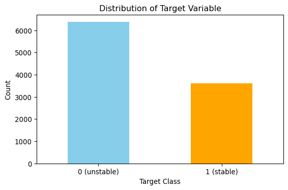

Train test split

Stratified sampling has been used to ensure the class proportions remain the same in the test and train sets.

from sklearn.model_selection import StratifiedShuffleSplit
from sklearn.preprocessing import StandardScaler

# Split the data
# Stratified sampling to help maintain similar distributions between the text and train sets
stratSplit = StratifiedShuffleSplit(n_splits=1, test_size=0.2, random_state=8)
for train_index, test_index in stratSplit.split(df.iloc[:, :-1], df["target"]):
    X_train = df.iloc[:, :-1].iloc[train_index]
    X_test = df.iloc[:, :-1].iloc[test_index]
    y_train = df["target"].iloc[train_index]
    y_test = df["target"].iloc[test_index]

# Fit scaler on training data
scaler = StandardScaler()
X_train_scald = scaler.fit_transform(X_train)

# Transform test data using the same scaler
X_test_scald = scaler.transform(X_test)

# check class distribution in test set
test_counts = y_test.value_counts()

# check null accuracy score
null_accuracy = (test_counts[0]/(test_counts[0] + test_counts[1]))

print(f"Null accuracy score: {null_accuracy:.4f}")

Null accuracy score: 0.6380

SVM

Here, support vector machine (SVM) models are fitted. The Support Vector Classifier (SVC) model in scikit learn has several hyperparameters. The hyperparameters can be divided into general and kernel-specific.

General SVM hyperparameters: * Kernel: Options are “linear”, “RBF”, “poly” and “sigmoid. * C: Regularisation parameter. Controls the trade-off between accuracy and generalisation. - High values create tighter decision boundaries (risk of overfitting).
- Low values allow smoother decision boundaries (risk of underfitting). * Class Weight: Useful for imbalanced datasets.

Kernel-specific hyperparameters: * “gamma”: Influence of individual data points. Available in “RBF”, “poly”, “sigmoid”. - Higher values make the model focus on local structures (risk of overfitting). - Lower values create smoother decision boundaries. * “coef0”: Controls curve shift in polynomial/sigmoid kernels. - Impacts feature interactions. * “degree”: Defines the complexity of polynomial curves. - Higher degrees create more flexible decision boundaries. * Class Weight: Useful for imbalanced datasets.

For this task, we have been asked to focus on:

• the kernel type - selecting three kernels.
• the regularisation parameter C.

I have performed hyperparameter optimisation to find the combination of parameters that gives the best model performance. For the model evaluation, I have used the weighted F1 score. F1 is the harmonic mean of precision and recall.

Kernel

For this section, I have focused on three kernels, “linear”, “poly” and “RBF”. For each kernel, I have performed hyperparameter optimisation to find the combination of parameters that gives the best model performance using the following parameters:

• “class_weight”: Applicable to all kernels.
• “gamma”: Applicable to “RBF” and “poly”.
• “coef0” and “degree”: Applicable only to “poly”.

All other hyperparameters not subject to the optimisation were left at their default values.

The search for optimal parameter combinations used the BayesSearchCV method. For each kernel, the best parameters are used to measure the model’s performance by plotting a confusion matrix and printing a summary of the accuracy, precision, recall and F1-score.

from skopt import BayesSearchCV
from sklearn.model_selection import StratifiedKFold, GridSearchCV
from sklearn.svm import SVC
from sklearn.metrics import accuracy_score, precision_score, recall_score, f1_score, confusion_matrix

# Create base search space
search_space = {"class_weight": [None, "balanced"]}

# RBF and poly specific parameters
rbf_search_space = {"gamma": (1e-4, 0.1, 'log-uniform')}

# Poly specific parameters
poly_search_space = {
    "degree": (2, 5),
    "coef0": (-1, 1)
}

# Define kernels
kernels = ["linear", "rbf", "poly"]

# Store results
results_kern = []

classes = ["0 (unstable)", "1 (stable)"]

cv = StratifiedKFold(n_splits=5)

for kernel in kernels:
    # Create model
    svc_model = SVC(kernel=kernel, probability=False, verbose=True, random_state=0)
    
    if kernel == "rbf":        
        search_space.update(rbf_search_space)
    elif kernel == "poly":
        search_space.update(poly_search_space)

    opt = BayesSearchCV(
        svc_model,
        search_spaces=search_space,
        scoring="f1_weighted",
        cv=cv,
        n_iter=10,  # Number of iterations
        n_jobs=-1,  # Use all cores
        verbose=0,
        random_state=0
    )

    opt.fit(X_train, y_train)  

    # Get best parameters from BayesSearch
    best_params = opt.best_params_
    print(f"\nHyperparameters {kernel}: {best_params}")
     
    # Train model using best parameters
    best_model_kern = SVC(kernel=kernel, random_state=0, **best_params)
    best_model_kern.fit(X_train, y_train)

    # Predict on test set
    y_pred = best_model_kern.predict(X_test)

    # Compute metrics
    accuracy = accuracy_score(y_test, y_pred)
    precision = precision_score(y_test, y_pred, average="weighted")
    recall = recall_score(y_test, y_pred, average="weighted")
    f1 = f1_score(y_test, y_pred, average="weighted")

    # Store results
    results_kern.append({
        "Kernel": kernel,
        "Accuracy": accuracy,
        "Precision": precision,
        "Recall": recall,
        "F1-score": f1,
        "Best Hyperparameters": best_model_kern.get_params()
    })

    # Plot Confusion Matrix
    cm = confusion_matrix(y_test, y_pred, labels=[0, 1])
    plt.figure(figsize=(6, 5))
    sns.heatmap(cm, annot=True, fmt="d", cmap="Blues", xticklabels=classes, yticklabels=classes)
    plt.xlabel("Predicted Labels")
    plt.ylabel("Actual Labels")
    plt.title(f"SVM Confusion Matrix - Kernel: {kernel}")
    plt.show()

# Convert results into a DataFrame
results_svm_kern_df = pd.DataFrame(results_kern)

[LibSVM]
Hyperparameters linear: OrderedDict([('class_weight', None)])

[LibSVM]
Hyperparameters rbf: OrderedDict([('class_weight', None), ('gamma', 0.04881101667405022)])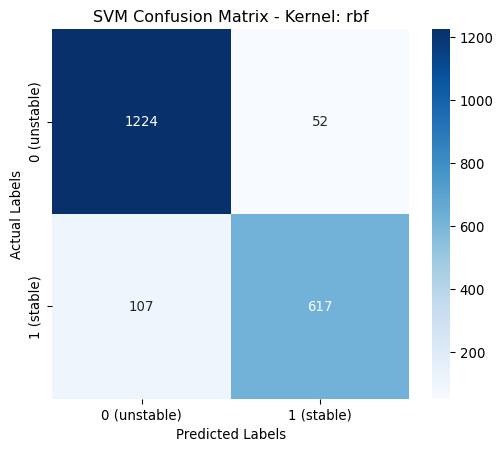

[LibSVM]
Hyperparameters poly: OrderedDict([('class_weight', None), ('coef0', 1), ('degree', 4), ('gamma', 0.06314005836673514)])

def print_performance_report_svm(df, param_keys_by_kernel):
    """
    Function to print a performance report.

    :param df: DataFame with performance data.
    :param param_keys_by_kernel: Dictionary with paramters keys to print for each kernel.
    :returns: None
    """
    # Columns to print directly
    selected_columns = ["Kernel", "Accuracy", "Precision", "Recall", "F1-score"]

    # Define column widths for alignment
    col_widths = {"K": 6, "A": 8, "P": 9, "R": 6, "F": 8}

    # Print a header
    print(f"Kernel | Accuracy | Precision | Recall | F1-score | Best Parameters (searched)")
    print("-" * 120)

    # Loop through the DataFrame and print each row horizontally
    for index, row in df.iterrows():
        kernel = row["Kernel"]
        selected_keys = param_keys_by_kernel.get(kernel, [])
        best_params_filtered = []
        for key in selected_keys:
            value = row["Best Hyperparameters"].get(key)
            if isinstance(value, float):
                formatted_value = f"{value:.4f}"
            else:
                formatted_value = str(value)
            best_params_filtered.append(f"{key}: {formatted_value}")
        line = f"{kernel:<{col_widths['K']}} | {row['Accuracy']:<{col_widths['A']}.4f} | {row['Precision']:<{col_widths['P']}.4f} | {row['Recall']:<{col_widths['R']}.4f} | {row['F1-score']:<{col_widths['F']}.4f} | {', '.join(best_params_filtered)}"
        print(line)

# Define which keys to print from best hyperparameters based on kernel value
param_keys_kernel = {
    "linear": ["classs_weights"],
    "rbf": ["classs_weights", "gamma"],
    "poly": ["classs_weights", "gamma", "degree", "coef0"]
}

# Display performance report
print("\nPerformance Report:")

print_performance_report_svm(results_svm_kern_df, param_keys_kernel)

Performance Report:
Kernel | Accuracy | Precision | Recall | F1-score | Best Parameters (searched)
------------------------------------------------------------------------------------------------------------------------
linear | 0.8250   | 0.8231    | 0.8250 | 0.8232   | classs_weights: None
rbf    | 0.9205   | 0.9206    | 0.9205 | 0.9198   | classs_weights: None, gamma: 0.0488
poly   | 0.9775   | 0.9775    | 0.9775 | 0.9775   | classs_weights: None, gamma: 0.0631, degree: 4, coef0: 1

From the above table it is shown that the poynomial kernel gives the best performance across all metrics.

Regularisation strength - C

# Create base search space
param_grid = {"C": [0.01, 0.1, 1, 10, 100, 1000]}

# Store results
results_C= []

# Dictionary to store cross-validation results.
scores = {}

for kernel in kernels:
    print(f"Kernel: {kernel}")

    # Get best parameters from previous section
    best_params_kern = results_svm_kern_df.loc[results_svm_kern_df["Kernel"] == kernel, "Best Hyperparameters"].values[0].copy()

    # Remove the "C", we are testing it here
    best_params_kern.pop("C", None)

    # Create model
    svc_model = SVC(**best_params_kern)

    # Set up GridSearchCV
    # GridSearchCV uses stratified sampling internally, so no special action is required.
    # Interested in performance for all classes, so use the macro option
    grid_search = GridSearchCV(svc_model, param_grid, cv=5, scoring="f1_weighted", n_jobs=-1,
                               return_train_score=True)

    # Fit the model
    grid_search.fit(X_train, y_train)

    # Store all results for this kernel
    scores[kernel] = grid_search.cv_results_

    # Get best parameters from GridSearch
    best_params_C = grid_search.best_params_

    # Add the best C to the current parameters    
    best_params = best_params_kern | best_params_C
 
    print(f"\nHyperparameters {kernel}: {best_params_C}")
     
    # Train model using best parameters
    best_model = SVC(**best_params)
    best_model.fit(X_train, y_train)

    # Predict on test set
    y_pred = best_model.predict(X_test)

    # Compute metrics
    accuracy = accuracy_score(y_test, y_pred)
    precision = precision_score(y_test, y_pred, average="weighted")
    recall = recall_score(y_test, y_pred, average="weighted")
    f1 = f1_score(y_test, y_pred, average="weighted")

    # Store results
    results_C.append({
        "Kernel": kernel,
        "Accuracy": accuracy,
        "Precision": precision,
        "Recall": recall,
        "F1-score": f1,
        "Best Hyperparameters": best_model.get_params()
    })

    # Plot Confusion Matrix
    cm = confusion_matrix(y_test, y_pred, labels=[0,1])
    plt.figure(figsize=(6, 5))
    sns.heatmap(cm, annot=True, fmt="d", cmap="Blues", xticklabels=classes, yticklabels=classes)
    plt.xlabel("Predicted Labels")
    plt.ylabel("Actual Labels")
    plt.title(f"SVM Confusion Matrix - Kernel: {kernel}")
    plt.show()

# Convert results into a DataFrame
results_svm_C_df = pd.DataFrame(results_C)

Kernel: linear

Hyperparameters linear: {'C': 1}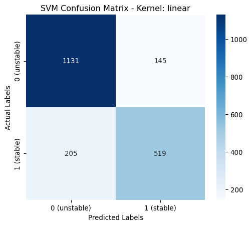

Kernel: rbf

Hyperparameters rbf: {'C': 100}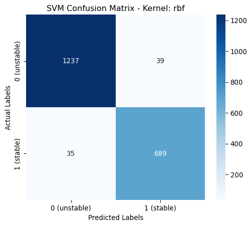

Kernel: poly

Hyperparameters poly: {'C': 0.1}

# Plotting the results
plt.figure(figsize=(10, 6))
for kernel, data in scores.items():
    plt.plot(data["param_C"], data["mean_test_score"], marker="o", label=kernel)

plt.xscale("log")
plt.xlabel("C value (log scale)")
plt.ylabel("Mean Validation Score")
plt.title("Comparision of mean validation score versus C value for different SVM kernels")
plt.legend()
plt.grid(True)
plt.tight_layout()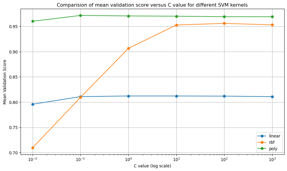

param_keys_C = {"linear": ["C" ], "rbf": ["C"], "poly": ["C"]}

# Display performance report
print("\nPerformance Report:")

print_performance_report_svm(results_svm_C_df, param_keys_C)

Performance Report:
Kernel | Accuracy | Precision | Recall | F1-score | Best Parameters (searched)
------------------------------------------------------------------------------------------------------------------------
linear | 0.8250   | 0.8231    | 0.8250 | 0.8232   | C: 1
rbf    | 0.9630   | 0.9631    | 0.9630 | 0.9630   | C: 100
poly   | 0.9755   | 0.9755    | 0.9755 | 0.9755   | C: 0.1000

Decision Tree

In this section, I train a decision tree and tune its depth. Decision trees have many hyperparameters, but for this exercise, the tuning is limited to “max_depth”. All other hyperparameters are left at their default values.

from sklearn.tree import DecisionTreeClassifier

# Create base search space
dt_param_grid = {"max_depth": range(1, 21)}

# Store results
dt_results= []

# Create model
dt_model = DecisionTreeClassifier(random_state = 0)

# Set up GridSearchCV
# GridSearchCV uses stratified sampling internally, so no special action is required.
# Interested in performance for all classes, so use the macro option
dt_grid_search = GridSearchCV(dt_model, dt_param_grid, cv=10, scoring="f1_weighted", n_jobs=-1,
                            return_train_score=True)

# Fit the model
dt_grid_search.fit(X_train, y_train)

# Store all results
dt_scores = dt_grid_search.cv_results_

# Get best parameters from GridSearch
dt_best_params = dt_grid_search.best_params_

print(f"\nHyperparameters: {dt_best_params}")
     
# Train model using best parameters
dt_best_model = dt_grid_search.best_estimator_

# Predict on test set
dt_y_pred = dt_best_model.predict(X_test)

# Compute metrics
dt_accuracy = accuracy_score(y_test, dt_y_pred)
dt_precision = precision_score(y_test, dt_y_pred, average="weighted")
dt_recall = recall_score(y_test, dt_y_pred, average="weighted")
dt_f1 = f1_score(y_test, dt_y_pred, average="weighted")

# Store results
dt_results.append({
    "Accuracy": dt_accuracy,
    "Precision": dt_precision,
    "Recall": dt_recall,
    "F1-score": dt_f1,
    "Best Hyperparameters": dt_best_model.get_params()
})

# Plot Confusion Matrix
dt_cm = confusion_matrix(y_test, dt_y_pred, labels=[0,1])
plt.figure(figsize=(6, 5))
sns.heatmap(dt_cm, annot=True, fmt="d", cmap="Blues", xticklabels=classes, yticklabels=classes)
plt.xlabel("Predicted Labels")
plt.ylabel("Actual Labels")
plt.title(f"Decision Tree Confusion Matrix")
plt.show()

# Convert results into a DataFrame
results_dt_df = pd.DataFrame(dt_results)

Hyperparameters: {'max_depth': 10}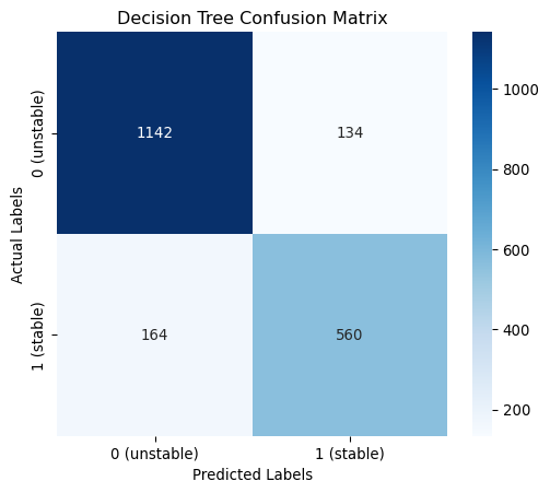

# Plotting the results
plt.figure(figsize=(10, 6))
plt.plot(dt_scores["param_max_depth"], dt_scores["mean_train_score"], marker="o", label="Training")
plt.plot(dt_scores["param_max_depth"], dt_scores["mean_test_score"], marker="o", label="Validation")

plt.xlabel("Tree-depth")
plt.ylabel("Mean Score")
plt.title("Accuracy comparison of training/validation set")
plt.legend()
plt.grid(True)
plt.tight_layout()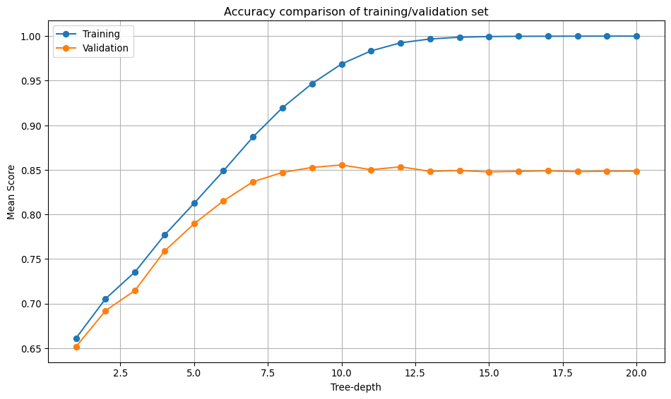

# Columns to print directly
selected_columns = ["Accuracy", "Precision", "Recall", "F1-score"]

# Define column widths for alignment
col_widths = {"A": 8, "P": 9, "R": 6, "F": 8}

# Print a header
print(f"Accuracy | Precision | Recall | F1-score | Best Parameters (searched)")
print("-" * 120)

# Loop through the DataFrame and print each row horizontally
for index, row in results_dt_df.iterrows():
    value = row["Best Hyperparameters"].get("max_depth")
    best_params_filtered = [f"max_depth: {value}"]
    line = f"{row['Accuracy']:<{col_widths['A']}.4f} | {row['Precision']:<{col_widths['P']}.4f} | {row['Recall']:<{col_widths['R']}.4f} | {row['F1-score']:<{col_widths['F']}.4f} | {', '.join(best_params_filtered)}"
    print(line)

Accuracy | Precision | Recall | F1-score | Best Parameters (searched)
------------------------------------------------------------------------------------------------------------------------
0.8510   | 0.8500    | 0.8510 | 0.8503   | max_depth: 10

Hyperparameter tuning

The Role of Hyperparameters

Hyperparameters are model settings that control the learning process and determine model complexity. Hyperparameters are not learned directly from the data. Hyperparameter tuning in model development is an important step that involves identifying the optimal model parameters. Proper hyperparameter tuning improves model accuracy, generalisation, and efficiency. Tuned hyperparameters prevent overfitting and underfitting by selecting an appropriate model complexity.

Model-Specific Impact: Different models have different hyperparameters. For SVMs, I tuned kernel-specific parameters (gamma, degree, coef0) and the regularisation parameter C. For Decision Trees, max_depth controls model complexity and overfitting.

Key Insights from my Results

Sequential vs. Joint Optimisation: My approach for SVM, which involves first optimising kernel-specific parameters with C=1, then optimising C separately, shows a common strategy. However, this sequential approach may not find the global optimum since parameters often interact. Joint optimisation using techniques like GridSearchCV or BayesSearchCV across all parameters simultaneously would likely yield better results.

Regularisation Effects (C parameter): - Linear kernel: C=1 was optimal, suggesting the default regularisation worked well. - RBF kernel: C=100 (less regularisation) improved performance significantly (0.9205 to 0.9630). - Polynomial kernel: C=0.1 (more regularisation) was optimal, preventing overfitting in this complex kernel.

Kernel Complexity Hierarchy: The results show the expected pattern: polynomial > RBF > linear in terms of model flexibility and performance on this dataset. The polynomial kernel achieved the highest performance (0.9775) but required strong regularisation (C=0.1).

Broader Hyperparameter Tuning Principles

Bias-Variance Tradeoff: Hyperparameters control the balance between model complexity and generalisation. The Decision Tree’s max_depth=10 represents finding the sweet spot between underfitting (too shallow) and overfitting (too deep).

Domain and Data Dependency: Optimal hyperparameters are highly dataset-dependent. The fact that different kernels required different C values demonstrates why systematic tuning is essential rather than using defaults.

Validation Strategy: Proper hyperparameter tuning requires robust validation (cross-validation) to ensure the selected parameters generalise well to unseen data, not just perform well on the training set.

Computational Efficiency: Tuning fewer parameters at a time reduces computational cost but may sacrifice optimality, but is likely to be better than using the defaults.