Data Cleaning and Text Analysis

# Versions of the libraries used are noted beside the import lines
# Python version: 3.11.7
import os
import time
import re
import pandas as pd                     # 2.1.4
import numpy as np                      # 1.26.4
import seaborn as sns                   # 0.12.2

import geopandas                        # 1.01
from geodatasets import get_path        # 2024.8.0
from geopy.geocoders import Nominatim   # 2.4.1
import matplotlib.pyplot as plt         # 3.8.0

from stop_words import get_stop_words   # 2018.7.23
import inflect                          # 7.5.0
from wordcloud import WordCloud         # 1.9.4
from IPython.display import Markdown    # 8.20.0
from collections import Counter 

import plotly.express as px             # 5.9.0
import textstat                         # 0.7.7

Introduction

The Stack Exchange site chosen for this analysis is the Quantitative (Quant) Finance (https://quant.stackexchange.com/) site. The Quant site is approximately 14.5 years old and has 62,000 users (May 2025). 23,000 questions have been asked, and 27,000 answers have been provided, with 74% of the questions being answered. On average, the is site receives 2.5 questions per day.

This document analyses the geographic distribution of the site’s users, the popular words used in posts, the popularity of tags used in posts, the type of programming language discussed and how this has change over the site’s life and the response time to answering questions, and some of the factors that may contribute to longer response times.

Privacy and Ethical Considerations

When conducting this analysis, several privacy and ethical concerns were given consideration. These were:

• Privacy concerns:
  • Unvalidated voluntary data: Users provide location information without verification, creating the potential for false data or privacy risks,
  • Geographic mapping: Converting user locations to precise latitude/longitude coordinates could enable identification of individuals, especially in smaller communities,
  • Data persistence: Location data from profiles may remain accessible long after users intend to share it.
• Ethical concerns:
  • Secondary use: Data was collected for Q&A purposes but is being used for research analysis,
  • Lack of explicit consent: Did users consent to geographic distribution analysis or behavioural profiling when creating accounts?
  • Data retention: Using archived data dumps raises questions about whether users can withdraw consent.

When mapping users’ locations, no user information (such as username, name, etc.) was stored with the calculated latitude and longitude coordinates, and the mapping was performed only to city, state, and country precision. Invalid locations were removed from the data. However, this doesn’t guarantee the location data is accurate.

Data

The data used in the analysis was downloaded from the site’s most recent data dump (2 May 2024) from https://archive.org/details/stackexchange/. The site data is contained in eight XML files containing information on badges, comments, post history, post links, posts, tags, users, and votes.

Convert data files from XML to CSV

The site’s data files are provided in XML format. The first step is to load each file separately and convert them to CSV. This is performed with the xml_to_csv function shown below. This step is only performed if the CSV file doesn’t exists to prevent performing the conversion each time the code is executed.

# Function to convert XML files to CSV
def xml_to_csv(file_name, csv_name=None, drop_cols=None):
    """
    Converts an XML file to CSV using Pandas.

    :param file_name: Name of the XML file to convert
    :param csv_name: Optional name of exported CSV file. If not provided, 
        the CSV file name will be the same as the XML file name.
    :param drop_cols: Optional list of columns to drop from dataframe
    """
    # Read XML file in dataframe
    df = pd.read_xml(file_name)

    # Check if the user wants to leave any columns out of the conversion
    if drop_cols is not None:
        for col in drop_cols:
            del df[col]
    # Set CSV name if not provided
    if csv_name is None:
        csv_name = file_name.split(".")[0]+ ".csv"
    # Write CSV file
    df.to_csv(csv_name, index=False)

    print(f"Converted {file_name} to {csv_name}")

# Convert the files if required
files = ["Badges", "Comments", "PostHistory", "PostLinks", "Posts", "Tags",
        "Users", "Votes"]

csv_files = []
for file in files:
    csv_file = os.path.join("data", file+".csv")
    xml_file = os.path.join("data", file+".xml")
    csv_files.append(csv_file)
    
    if os.path.exists(csv_file):
        print(f"File '{csv_file}' exists.")
    else:
        print(f"File '{csv_file}' does not exist.")
        xml_to_csv(xml_file,drop_cols=drops[file])

Load CSV data files into pandas data frames

Each CSV file is loaded into pandas data frames. For each data frame, the datatype (dtype) was checked (not shown in the code), and corrections were made if pandas incorrectly assigned the data type. Corrections were often needed for DateTime fields and some string fields.

# Load the data from CSV file into pandas data frames
badges = pd.read_csv(csv_files[0], comment="#")

# Correct data types in data frame
badges["Date"] = pd.to_datetime(badges["Date"])
badges = badges.astype({"Name": "string"})

# Load the data from CSV file into pandas data frames
comments = pd.read_csv(csv_files[1], comment="#")

# Correct data types in data frame
comments["CreationDate"] = pd.to_datetime(comments["CreationDate"])
comments = comments.astype({"Text": "string", "UserDisplayName":"string"})

# Load the data from CSV file into pandas data frames
post_history = pd.read_csv(csv_files[2], comment="#")

# Correct data types in data frame
post_history = post_history.convert_dtypes()
post_history["CreationDate"] = pd.to_datetime(post_history["CreationDate"])

# Load the data from CSV file into pandas data frames
post_links = pd.read_csv(csv_files[3], comment="#")

# Correct data types in data frame
post_links["CreationDate"] = pd.to_datetime(post_links["CreationDate"])

# Load the data from CSV file into pandas data frames
posts = pd.read_csv(csv_files[4], comment="#")

# Correct data types in data frame
posts = posts.convert_dtypes()
posts["CreationDate"] = pd.to_datetime(posts["CreationDate"])
posts["LastEditDate"] = pd.to_datetime(posts["LastEditDate"])
posts["LastActivityDate"] = pd.to_datetime(posts["LastActivityDate"])
posts["CommunityOwnedDate"] = pd.to_datetime(posts["CommunityOwnedDate"])
posts["ClosedDate"] = pd.to_datetime(posts["ClosedDate"])

# Load the data from CSV file into pandas data frames
tags = pd.read_csv(csv_files[5], comment="#")

# Correct data types in dataframe
tags = tags.convert_dtypes()

# Load the data from CSV file into pandas data frames
users = pd.read_csv(csv_files[6], comment="#")
users.head()

# Correct data types in dataframe
users = users.convert_dtypes()
users["CreationDate"] = pd.to_datetime(users["CreationDate"])

# Load the data from CSV file into pandas data frames
votes = pd.read_csv(csv_files[7], comment="#")
votes.head()

# Correct data types in dataframe
votes["CreationDate"] = pd.to_datetime(votes["CreationDate"])

Analysis

Geographic distribution of forum users

This section investigates the distribution of forum users worldwide by using the location information provided by users on their account profiles. The location information users enter is optional, and no form of validation is performed. This results in many empty entries and free-form input of the data. The free-form input presents challenges when working with the data. These challenges are identified and addressed in this section, while others remain for future improvements.

Data clean-up

Remove any rows in the users data frame that do not contain location information.

num_users = users.shape[0]
# Drop rows that have no location
users.dropna(subset=["Location"], inplace=True)
num_users_loc = users.shape[0]

In May 2024, 50776 users of the Quant site were registered, and 14636 of these had provided an entry in the location field of their profile.

The next step is to determine how many of the provided locations contain valid information that can be used to locate the user on a map. This is an issue of privacy, so Stack Exchange does not require users to provide a location. Privacy could also be the reason the location provided is not validated.

A function was created to validate the location. To be a valid location, the string must contain either of the following patterns: “city, state, country” or “city, country”. The functions start by checking if the string only contains numbers, URLs or non-ASCII characters. Then, it checks if any invalid character sequences have been found, such as double hyphens, double apostrophes, etc. A name pattern is used for each valid name component and accepts letters, spaces, hyphens, apostrophes and periods. This pattern is compiled into a full pattern that adds commas and spaces between each name.

The captured groups from the regex match are then checked to ensure that the city isn’t empty and the state isn’t empty if a country is provided. If only the city were state are provided, the state could also represent the country, e.g., Paris, France. If only a city and state are provided, this could also be for an American user as they often don’t enter their country. It has been observed that some invalid locations are still allowed by the function, and therefore, the function could be improved.

def is_valid_location(location_string):
    """
    Uses regex to validate if a location string follows the pattern of:
    - 'city, state, country' OR 
    - 'city, country' (valid for no USA countries or USA locations)
    
    Rejects strings with only numbers, URLs, non-ASCII characters.
    Rejects invalid character sequences:
        - Double hyphens
        - Double apostrophes
        - Hyphen followed by apostrophe
        - Apostrophe followed by hyphen
        - Double periods

    A name pattern is used to identify valid name components 
    (city, state, country). This pattern now accepts letters, spaces,
     hyphens, apostrophes, and periods.

    The function requires at least two matches of the name pattern and marks
    any entries were the state and 'usa'/'united states' are not separated
     by a comma as invalid

    This function allows some invalid locations, therefore could be improved.
    
    :param location_string: String containing the location information to check
    :return: True or False depending on if the location_string is valid
    """
    # Clean up input string
    location_string = location_string.strip()
    
    # Reject if contains URLs, or non-ASCII characters
    if re.search(r"^[\d\s]+$|http|www|[^\x00-\x7F]", location_string):
        return False

    # Check for invalid character patterns
    invalid_patterns = {
    "double_hyphen": re.compile(r"--"),      # Double hyphens
    "double_apostrophe": re.compile(r"''"),  # Double apostrophes
    "hyphen_apostrophe": re.compile(r"-'"),  # Hyphen followed by apostrophe
    "apostrophe_hyphen": re.compile(r"'-"),  # Apostrophe followed by hyphen
    "double_period": re.compile(r"\.\.")     # Double periods
    }

    # Check for invalid character sequences
    for pattern_name, pattern in invalid_patterns.items():
        if pattern.search(location_string):
            return False

   
    # Define pattern for valid name components (city, state, country)
    # This pattern now accepts letters, spaces, hyphens, apostrophes, and
    #  periods.
    name_pattern = r"[A-Za-z\s\-'.]+"

    # Build the full pattern using the name_pattern
    location_pattern = re.compile(
        f"^({name_pattern}),\\s*({name_pattern})(?:,\\s*({name_pattern}))?$"
    )

    match = re.match(location_pattern, location_string)
    if not match:
        return False

    # Extract the captured groups
    groups = match.groups()
    city = groups[0].strip()
    state = groups[1].strip()
    country = groups[2].strip() if groups[2] else None
    
    # Ensure city and state are not empty
    if not city or not state:
        return False
        
    # If we have a country part (3-part format), ensure it's not empty
    if groups[2] is not None and not country:
        return False

    substrings = ["usa", "us", "united states"]
    # Any entries that state == USA are dropped
    if state.lower() in substrings:
        return False

    # Check the we don't have other strings with the substrings
    for substring in substrings:
        if substring in state.lower():
            return False
        
    # Passed all checks
    return True

The is_valid_location function is applied to the Location column of the users data frame, with the function output captured in a new column, ValidLocation. Users without a valid location are removed from the analysis as a latitude and longitude cannot be found for invalid locations.

# Apply is_valid_location function to the dataSeries Location
users["ValidLocation"] = users["Location"].apply(is_valid_location)

# Drop rows without a valid location
users = users[users["ValidLocation"]]
num_users_valid_location = users.shape[0]

The number of users with valid locations is 7598.

Now that valid locations have been found, the next step is to take the location information and separate it into city, state, and country for usage later. For this purpose, a function was created to extract the location parts from the location string. The function extract_location_parts takes a string and splits it into parts at commas. If the split produces three parts, they are assumed to represent the city, state, and country. If, after the split, only two parts are obtained, then it is assumed the first part represents the city. The second part is checked to see if it matches any American state or territory; if it does, then the second part is assigned to the state and the country is set to “USA”. If the second part doesn’t match any American state or territory, it is assumed to represent a country and the state is set to None. This function could be improved further by adding a check to the country part, making sure it is a valid country.

def extract_location_parts(location_string):
    """
    Extract the parts of a location as city, state, country from a provided
     string.

    :param location_string: String to get location parts from
    :return: pandas data series containing the parts of the location
    """
    # Split the input string by commas
    parts = [part.strip() for part in location_string.split(",")]

    # Check if already in city, state, country format
    if len(parts) == 3:
        city, state, country = parts
    
    # Check if in city, country or city, state format
    elif len(parts) == 2:
        city, second_part = parts
        
        # Check if the second part might be a US state
        #us_states = {"AL", "AK", "AZ", "AR", "CA", "CO", "CT", "DE", "FL", "GA", 
        #             "HI", "ID", "IL", "IN", "IA", "KS", "KY", "LA", "ME", "MD", 
        #             "MA", "MI", "MN", "MS", "MO", "MT", "NE", "NV", "NH", "NJ", 
        #             "NM", "NY", "NC", "ND", "OH", "OK", "OR", "PA", "RI", "SC", 
        #             "SD", "TN", "TX", "UT", "VT", "VA", "WA", "WV", "WI", "WY",
        #             "DC"}  # Adding District of Columbia
        us_states = {
        # https://en.wikipedia.org/wiki/
        # List_of_states_and_territories_of_the_United_States#States.
            "AK", "AL", "AR", "AZ", "CA", "CO", "CT", "DE", "FL", "GA",
            "HI", "IA", "ID", "IL", "IN", "KS", "KY", "LA", "MA", "MD",
            "ME", "MI", "MN", "MO", "MS", "MT", "NC", "ND", "NE", "NH",
            "NJ", "NM", "NV", "NY", "OH", "OK", "OR", "PA", "RI", "SC", 
            "SD", "TN", "TX", "UT", "VA", "VT", "WA", "WI", "WV", "WY",
        # https://en.wikipedia.org/wiki/
        # List_of_states_and_territories_of_the_United_States#Federal_district.
            "DC",
        # https://en.wikipedia.org/wiki/
        # List_of_states_and_territories_of_the_United_States
        # #Inhabited_territories.
            "AS", "GU", "MP", "PR", "VI",
        }
        
        # Also check for full state names
        us_state_names = {
        # https://en.wikipedia.org/wiki/
        # List_of_states_and_territories_of_the_United_States#States.
            "Alabama", "Alaska", "Arizona", "Arkansas", "California", 
            "Colorado", "Connecticut", "Delaware", "Florida", "Georgia", 
            "Hawaii", "Idaho", "Illinois", "Indiana", "Iowa", "Kansas", 
            "Kentucky", "Louisiana", "Maine", "Maryland", "Massachusetts", 
            "Michigan", "Minnesota", "Mississippi", "Missouri", "Montana", 
            "Nebraska", "Nevada", "New Hampshire", "New Jersey", "New Mexico", 
            "New York", "North Carolina", "North Dakota", "Ohio", "Oklahoma", 
            "Oregon", "Pennsylvania", "Rhode Island", "South Carolina", 
            "South Dakota", "Tennessee", "Texas", "Utah", "Vermont", 
            "Virginia", "Washington", "West Virginia", "Wisconsin", "Wyoming",
        # https://en.wikipedia.org/wiki/
        # List_of_states_and_territories_of_the_United_States#Federal_district.        
            "District of Columbia",
        # https://en.wikipedia.org/wiki/
        # List_of_states_and_territories_of_the_United_States
        # #Inhabited_territories.
            "American Samoa", "Guam GU", "Northern Mariana Islands",
            "Puerto Rico PR", "U.S. Virgin Islands"
        }

        # If the second part looks like a US state, treat it as city, state and
        #  add USA
        if second_part.upper() in us_states or second_part in us_state_names:
            state = second_part
            country = "USA"
        else:
            # Otherwise, it's city, country format
            country = second_part
            state = None
    
    return pd.Series([city, state, country])

The extract_location_parts function is applied to the Location column of the user data frame and the result is returned as three new columns: city, state, and country. For ease of processing, a copy of the users data frame is produced that only contains unique entries for the city, state, and country.

users[["City", "State", "Country"]] = users["Location"].apply(
    extract_location_parts)

users_geo = users.drop_duplicates(
    subset=["City","State","Country"])[["City", "State", "Country"]].copy()
num_unique_loc = users_geo.shape[0]

After cleaning the user’s location data 2000 unique locations required geo-locating.

Obtaining latitude and longitude

The geopy package is used to obtain the latitude and longitude of a location . Geopy provides a client interface for several popular geocoding web services. The Nominatim web service was utilised as it is free. Nominatim uses OpenStreetMap data to find locations on Earth by name and address. The only limitations found were that it required only one request per second and could time out. A time out value of 60 seconds was found to work.

def get_lat_lon(city, country, state=None):
    """
    Function to return the latitude and longitude given a city, state,
     country or city, country. If no latitude or longitude can be 
     found for the provided address then None is returned.

    :param city: string containing the name of locations city
    :param country: string containing the name of locations country
    :param state: Option string containing the name of locations state
    :return: Pandas data series containing the latitude and longitude
    """
    geolocator = Nominatim(user_agent="geocoder")

    # Slow down the requests. The Nominatim usage policy says no more than one
    #  request per second
    time.sleep(1.1)
    
    if state:
        location = geolocator.geocode(f"{city}, {state}, {country}", timeout=60)
    else:
        location = geolocator.geocode(f"{city}, {country}", timeout=60)
        
    if location:
        return pd.Series([location.latitude, location.longitude])
    else:
        return pd.Series([None, None])

Since the requesting latitude and longitude for each location was slow, it was only performed once, and the result was stored on disk. If the user_geolocation.csv file is found on disk, then the data is loaded into a data frame. Otherwise, it is calculated and stored on disk.

geo_location_file = os.path.join("data", "user_geolocation.csv")
if os.path.exists(geo_location_file):
    print(f"File '{geo_location_file}' exists.")
    print(f"Reading geo locations.")
    users_geo = pd.read_csv(geo_location_file, comment="#")
else:
    print(f"File '{geo_location_file}' does not exist.")
    print(f"Creating geo locations.")
    users_geo[["Latitude","Longitude"]] = users_geo.apply(
        lambda x: get_lat_lon(x["City"], x["Country"],x["State"]), axis=1)

    # Drop and location where a latitude or longitude was not found
    users_geo = users_geo.dropna(subset=["Latitude", "Longitude"])
    users_geo.to_csv(geo_location_file, index=False)

num_unique_loc_val = users_geo.shape[0]
num_invalid_latlong = num_unique_loc - num_unique_loc_val

Due to false positives in the cleaning function, there were still some (71) invalid locations were a latitude and longitude did not exist. Thus the final number of unique user locations was 1929.

Producing a map of locations

The unique user locations were plotted onto a world map using Geopandas.

gdf = geopandas.GeoDataFrame(
    users_geo, geometry=geopandas.points_from_xy(
        users_geo.Longitude, users_geo.Latitude), crs="EPSG:4326"
)

world = geopandas.read_file(get_path("naturalearth.land"))

fig = plt.figure(figsize=(12, 6))
ax = fig.add_subplot()

# Remove Antarctica
world.clip([-180, -55, 180, 90]).plot(
    ax=ax, color="lightgray", edgecolor="black")

# We can now plot our GeoDataFrame.
gdf.plot(ax=ax, color="red", markersize=8)
ax.set_xticks([])
ax.set_yticks([])
plt.title("Location of Quant Stack Exchange users")
plt.show()

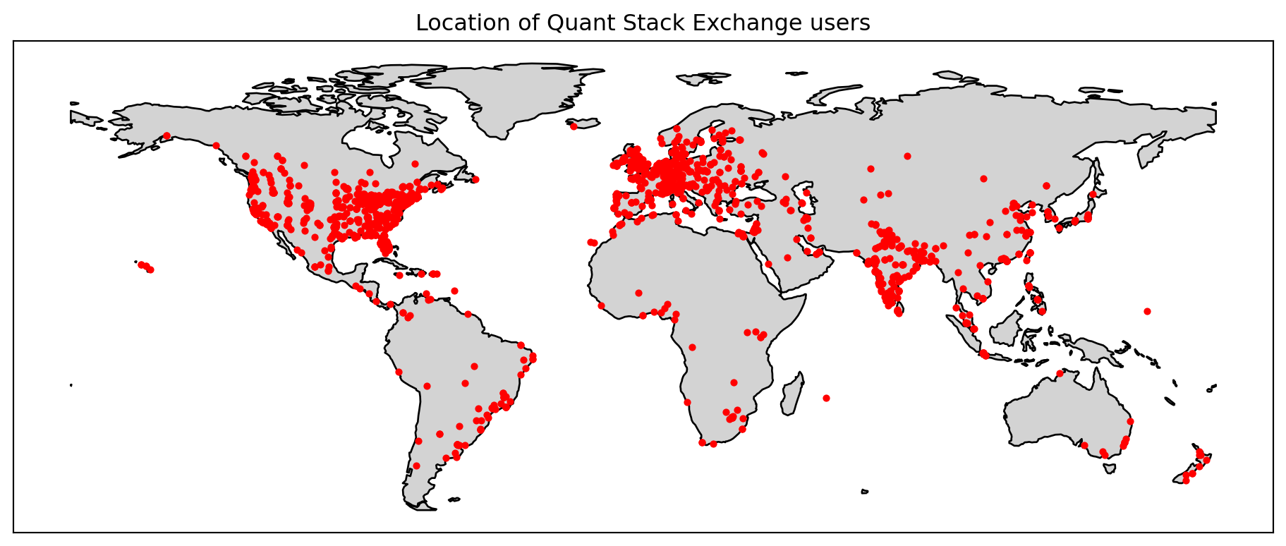
Figure 1: Location of Quant Stack Exchange users

Figure 1 shows the unique locations of the Quant Stack Exchange site users worldwide. Many users are clustered in Europe, the east and west coasts of the United States and India. Africa, South America and South-East Asia have fewer user sites. In Australia, the users are located around capital cities, with Perth being an exception, with no users.

The top 100 words used in the titles of the top 20% of questions

For this analysis, the titles of questions are analysed for the top 20% of posts based on their score, and the top 100 words are extracted and visualised as a word cloud. The count of the top 20 words are shown in a table. A post’s score is the number of UpVotes minus the number of DownVotes.

Data preparation

To prepare the data for visualisation, a data frame consisting of only questions is created from the posts data frame using the PostTypeId column. Questions have a PostTypeId = 1. A function (text_clean) is created that will clean the title text for each post. The cleaning involves converting all text to lowercase, removing any numbers, removing common words (stop words), and converting plurals to the singular version. The text_clean function is applied to the Title column from the questions data frame, and the result is returned as a new column, CleanTitle. The questions data frame is then filtered only to have posts with a score higher than the top 80% of scores. Cleaned titles from the remaining posts are converted to a list.

# Filter for questions only (PostTypeId = 1)
# Make a copy as we modify this data frame later
questions = posts[posts["PostTypeId"] == 1].copy()

# Generic English stop words to ignore
stop_words = get_stop_words("en")

# Define custom stop words for the finance domain
custom_stopwords = ["can", "question", "using", "use", "value", "values",
        "calculate", "formula", "formulas", "quant", "quantitative",
        "finance", "financial"]

# Combine generic and custom stop words
stop_words.extend(custom_stopwords)

# Function to clean text
def clean_text(text, convert_plurals=False):
    # Convert to lowercase
    text = text.lower()
    
    # Remove numbers
    text = re.sub(r"\d+", "", text)
    
    # Remove stop words
    words = [word for word in text.split() 
            if word not in stop_words and len(word) > 2]

    # Convert plurals of words to their singular form
    if convert_plurals:
        p = inflect.engine()
        words = [p.singular_noun(word) 
                if p.singular_noun(word) else word  for word in words]
    
    return " ".join(words)

# Clean the titles
questions["CleanTitle"] = questions["Title"].apply(
    clean_text,  convert_plurals=True)

# Separate high posts
high_posts = questions[questions["Score"] >= questions["Score"].quantile(0.8)]

# Combine all titles for each group
high_posts_text = " ".join(high_posts["CleanTitle"].tolist())

Visualisation and Top 20 words

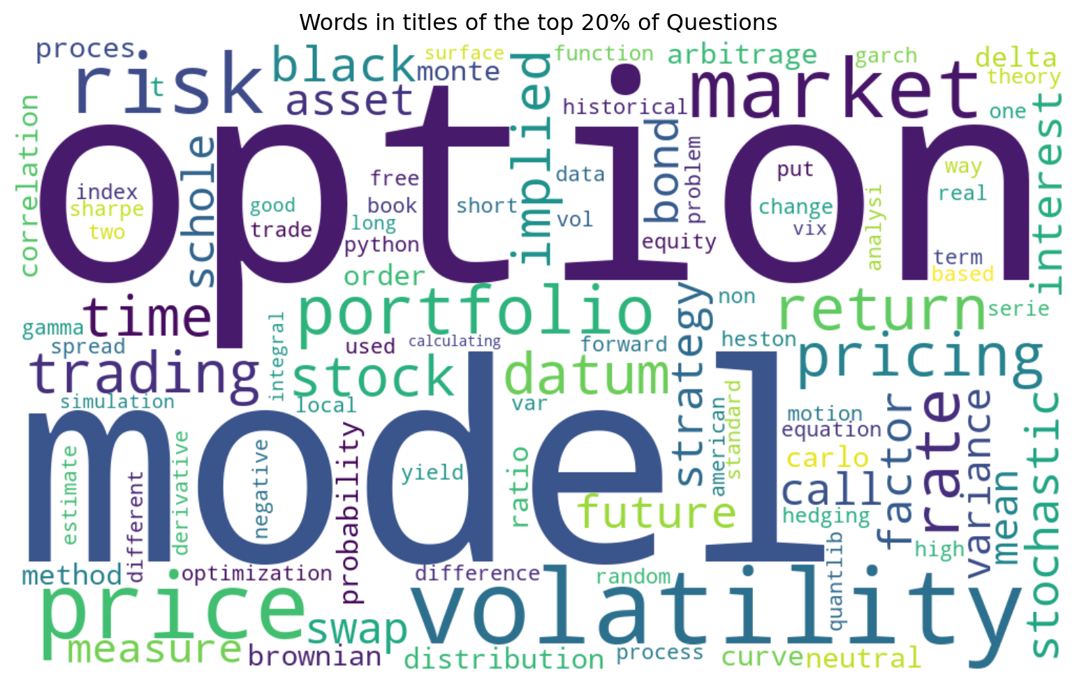
Figure 2 shows the words used in the titles of the 20% of the questions. Option, model and volatility are the words that stand out. It isn’t surprising that “option” was the most common occurring word in the questions, given it is the most used type of derivative by financial markets. Table 1 shows the top 20 words that appear in the high-scoring posts. It is observed that the words are those that you would expect from financial discussions. The words I would have expected to see but are missing are those relating to programming, programming languages and specific financial models such as the black-scholes.

# Generate word cloud for the top 100 words
wordcloud = WordCloud(width=1000, height=600, background_color="white",
        max_words=100, collocations=False, contour_width=3
        ).generate(high_posts_text)
    
plt.figure(figsize=(10, 5))
plt.imshow(wordcloud, interpolation="bilinear")
plt.axis("off")
plt.tight_layout()
plt.title("Words in titles of the top 20% of Questions")
plt.show()

Figure 2: Words in titles of the top 20% of Questions

# Analyse word frequencies
high_freq = Counter(high_posts_text.split())

# Get the most common words in each category
df = pd.DataFrame(high_freq.most_common(20), columns=["Word","Count"])
Markdown(df.to_markdown(index = False))

Table 1: Top 20 words in the title of the high-scoring questions

Word	Count
option	419
volatility	383
model	364
price	282
portfolio	234
market	223
rate	199
datum	190
pricing	183
risk	174
return	171
stock	158
implied	154
trading	154
time	135
stochastic	118
future	107
bond	100
interest	100
factor	91

Evolution of tag popularity over time

This visualisation tracks how the popularity of different tags changes over time. Tags are used to categorise posts, making it easier for people to search for posts related to a particular topic.

Data preparation

The first step is to drop any rows that contain a NaN in the Tags column of the posts data frame. The return from this operation is a view into the data frame, which will prevent the addition of any new columns. Therefore, a copy (posts_cleaned) of the data frame is made to allow for alteration. The tags for each post are stored as |tag1|tag2|tag3| etc. A function, separate_tags, was created to separate the tags from a string to a list of individual tags with this format. The separate_tags function is applied to the posts_cleaned data frame, and the results are stored in a new column called SepTag. Having the tags in a list isn’t helpful for visualisation, so the explode function creates duplicate rows for each tag in the list of a given row (tag_posts). The creation date for the posts is used to create a new column containing each post’s month-year. The data is then grouped by month and tag to allow for counting occurrences of each tag per month. The top ten tags by count are extracted into a list, which is then used to filter the monthly tag counts so only the top ten tags remain. The last step is to create a column in the posts_cleaned data frame for the tag type. If the SepTags column is empty, then the ‘No Tag’ label is applied; if the tag lists contain any of the top 10 tags, the label’ Popular Tag’ is applied; otherwise, the label ‘Unpopular Tag’ is applied. These labels will be used in later visualisations.

# Drop rows with NA values in the Tags column and make a copy of the resulting
#  data frame
posts_cleaned = posts.dropna(subset=["Tags"]).copy()

# Tags in StackExchange are stored as |tag1|tag2|tag3|
def separate_tags(x):
    """
    Function to separate tags and return as a list

    :param x: string containing tags that need separating
    :return: A list of tags 
    """
    return x[1:-1].split("|")

# Apply the separate_tags function to the "Tags" column and store the result
#  in a new column
posts_cleaned["SepTag"] = posts_cleaned["Tags"].apply(separate_tags)

# Use explode to ensure that there is only one tag per row. This duplicates 
# rows for all other column values
tag_posts = posts_cleaned.explode("SepTag")

# Group by month and tag to count occurrences
tag_posts["Month"] = tag_posts["CreationDate"].dt.to_period("M")
monthly_tag_counts = tag_posts.groupby(
    ["Month", "SepTag"]).size().reset_index(name="Count")

# Convert Period to datetime for plotting
monthly_tag_counts["MonthDate"] = monthly_tag_counts["Month"].dt.to_timestamp()

# Get the top 10 tags
top_tags = tag_posts["SepTag"].value_counts().nlargest(10).index.tolist()

# Filter for only the top tags
top_tag_counts = monthly_tag_counts[monthly_tag_counts["SepTag"].isin(top_tags)]

# Define conditions and choices
conditions = [
    # Empty list check
    posts_cleaned["SepTag"].str.len() == 0,  
    # Intersection check
    posts_cleaned["SepTag"].apply(lambda x: bool(set(x) & set(top_tags)))  
]

# Create a TagType column
choices = ["No Tag", "Popular Tag"]
posts_cleaned["TagType"] = np.select(
    conditions, choices, default="Unpopular Tag")

Visualisation of the top 10 tags

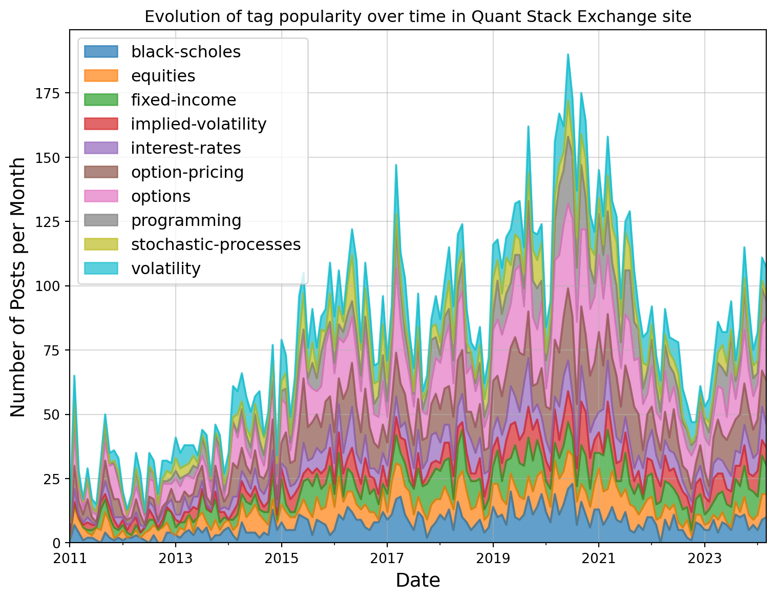
For the visualisation, a stacked area chart is chosen as it allows to see the cumulative total of the top 10 tags as well as their distribution. Figure 3 shows the evolution of the tag’s popularity over time.

# Create a pivot table for the stacked area chart
pivot_data = top_tag_counts.pivot(
    index="MonthDate", columns="SepTag", values="Count")

# Create the visualization
plt.rcParams["figure.figsize"] = (8,6)

# Stacked area chart
ax = pivot_data.plot.area(alpha=0.7)
plt.xlabel("Date", fontsize=14)
plt.ylabel("Number of Posts per Month", fontsize=14)

# Add a legend
ax.legend(loc="upper left", fontsize=12)
plt.tight_layout()
plt.title("Evolution of tag popularity over time in Quant Stack Exchange site")
plt.grid(True, alpha=0.5)
plt.show()

Figure 3: Evolution of tag popularity over time in Quant Stack Exchange site

Some observations from this graph:

• From 2011 to 2021, the monthly posts increased, although there were some sudden drops between 2016 and 2021. This might be attributed to periods of global economic challenges, such as the financial challenges in 2018. It was a year marked by market volatility, economic concerns, and a slowdown in growth, making it a challenging period for investors and the global economy.
• The number of monthly posts declined from 2021 to the end of 2022. This period was during the COVID-19 pandemic. Was this decline related to COVID-19 or some other reasons?
• Monthly posts have increased since 2023 but not back to the level of 2021.
• ChatGPT launched at the end of 2022. Does this affect why the number of posts hasn’t recovered since 2023? Are people now asking Chatgpt for answers rather than posting on the Quant Stack Exchange site?
• From 2011 to 2024, the most common tags were options, options pricing, and black scholes, which are the mathematical equations used to price options.
• Programming was not popular in the early years, but has gained popularity since, especially during the COVID-19 period.
• ‘Volatility’ appears more often in the word cloud than in the tag usage. ‘Black-scholes’ appears in the top 10 tags but not in the top 20 title words. This implies users are using tag words in post titles but not tagging the posts with an appropriate tag, or they are tagging posts but not using the the tag words in the title. Therefore, if title words and tags are isolated, they are not good indicators of what topic the post is about.

Cross-site reference analysis for the top 25 domains

Data preparation

A regular expression pattern is used to find all occurrences of ‘http’ or ‘https’ followed by ‘://’, followed by words, hyphens and periods. The regular expression pattern is used with the pandas findall command on the Body column of the posts data frame. The results from the findall matching are returned as a list and stored in a new column called Domains. Similar to the tags processing, the data frame is exploded using the list entries in the Domains column, and the unique domain names are counted and returned as a data series in descending order. The domains are then classified as an internal domain, a link to another stack exchange site or stackoverflow, or an external domain. The top 25 domains and counts are then copied into another data frame for further processing. The total counts of each type are calculated, and then for each domain its percentage of type count and percentage of the overall count is evaluated.

# Regular expression for finding URL's in posts r"https?://([\w\-\.]+)"
  # https? - matches http or https
  # :// - matches the colon and two forward slashes
  # ([\w\-\.]+) - Group to match domain name.
    # [] character class
      # \w match any word (alphanumeric + underscore)
      # \- match a hyphen
      # \. match a period/dot
      # + - make the match greedy and allow one or match of the character class
pattern = r"https?://([\w\-\.]+)"

# Find all patterns and return as a list stored in new column Domains.
posts["Domains"] = posts["Body"].str.findall(pattern)

# Use explode to create new rows for each entry in the lists in the domains
#  column
# Select the domains column and count the unique entries. The data series will 
# be returned sorted in descending order
# Reset the index
domain_counts = posts.explode(
    "Domains")["Domains"].value_counts().reset_index().rename(
        columns={"count":"Count"})

# Classify the domains as internal or external using a regular expression 
# search for domain names
# Any stackexchange or stackoverflow domains are internal 
# (r"stackexchange|stackoverflow")
domain_counts["Type"] = domain_counts["Domains"].str.contains(
    r"stackexchange|stackoverflow", case=False, regex=True).map(
        {True: "Internal", False: "External"})

# Get the top 25 domains
# Make a copy so we can add extra columns later
top_25_domains = domain_counts.head(25).copy() 

# Calculate total counts by type
domain_type_totals = top_25_domains.groupby("Type")["Count"].transform("sum")

# Calculate the overall total
total_links = top_25_domains["Count"].sum()

# Add percentage columns
top_25_domains["Percentage of Type"]= (
    top_25_domains["Count"] / domain_type_totals * 100).round(2)
top_25_domains["Percentage Overall"] = (
    top_25_domains["Count"] / total_links * 100).round(2)

# Sort by type and count (descending)
top_25_domains = top_25_domains.sort_values(
    ["Type", "Count"], ascending=[True, False])

Summary table and tree map for the top 25 domains

posts_total = posts["Body"].shape[0]
posts_total_links = domain_counts.shape[0]
avg_links_post = round(total_links/posts_total_links)

Summary information for the cross-site data analysis:

• Total number of posts (questions and answers): 48764
• Total number of posts with website links: 4726
• Total number of website links: 21210
• Average links per post with any links: 4

Approximately 10% of posts have website links. When a post has a link, the average number of links is 4.

def colour_rows_by_type(row):
    """
    Function to set the background colour for a row based upon its domain type

    :param row: Row to return background colour for
    :return: List of background colours for each entry in the row
    """
    if row["Type"] == "Internal":
        # Light blue for Internal
        return ["background-color: #E6F2FF"] * len(row)  
    else:
        # Light red for External
        return ["background-color: #FFECE6"] * len(row)  

# Apply the styling and hide the index
styled_table = top_25_domains.style.apply(
    colour_rows_by_type, axis=1).hide(axis="index")

# Basic styling
styled_table = styled_table.format({"Count": "{:,d}",
    "Percentage of Type": "{:.2f}%",
    "Percentage Overall": "{:.2f}%"
})

# Add a table style with borders
styled_table = styled_table.set_table_styles([
    {"selector": "th", "props": [("background-color", "#f5f5f5"), 
                                ("color", "#333"), 
                                ("font-weight", "bold"),
                                ("border", "1px solid #ddd"),
                                ("padding", "8px")]},
    {"selector": "td", "props": [("border", "1px solid #ddd"),
                                ("padding", "8px")]},
    {"selector": "caption", "props": [("caption-side", "top"), 
                                     ("font-size", "16px"),
                                     ("font-weight", "bold"),
                                     ("color", "#333")]}
])

styled_table

Table 2: Domain Count, Type and Percentages coloured by type

Domains	Count	Type	Percentage of Type	Percentage Overall
i.stack.imgur.com	9,163	External	51.49%	43.20%
en.wikipedia.org	2,945	External	16.55%	13.88%
papers.ssrn.com	1,073	External	6.03%	5.06%
github.com	779	External	4.38%	3.67%
arxiv.org	589	External	3.31%	2.78%
www.cmegroup.com	294	External	1.65%	1.39%
www.investopedia.com	284	External	1.60%	1.34%
cran.r-project.org	281	External	1.58%	1.32%
ssrn.com	252	External	1.42%	1.19%
www.sciencedirect.com	245	External	1.38%	1.16%
www.sec.gov	241	External	1.35%	1.14%
finance.yahoo.com	220	External	1.24%	1.04%
onlinelibrary.wiley.com	210	External	1.18%	0.99%
doi.org	202	External	1.14%	0.95%
www.jstor.org	196	External	1.10%	0.92%
www.youtube.com	178	External	1.00%	0.84%
www.google.com	175	External	0.98%	0.83%
www.researchgate.net	169	External	0.95%	0.80%
www.bloomberg.com	151	External	0.85%	0.71%
www.quandl.com	149	External	0.84%	0.70%
quant.stackexchange.com	2,286	Internal	66.96%	10.78%
rads.stackoverflow.com	590	Internal	17.28%	2.78%
stats.stackexchange.com	210	Internal	6.15%	0.99%
math.stackexchange.com	191	Internal	5.59%	0.90%
stackoverflow.com	137	Internal	4.01%	0.65%

Table 2 shows the domain counts, type and percentages. Observations of this data:

• 16 % of the links in posts are to other Stack Exchange or Stack Overflow sites, i.e., they are internal.
• Of the internal links, 67 % are self-links to other posts within the Quant Stack Exchange site, https://quant.stackexchange.com.
• The remaining 84% of links are to external websites, with a majority of these being sites that host academic publications such as https://papers.ssrn.com, https://arxiv.com, https://www.jstor and https://www.researchgate.net
• All images in Stack Exchange posts are hosted from https://i.stack.imgur.com. That’s why this domain makes up 43.2% of the post links.

Approximately 10% of the posts website links, and 43% are images.

The tabular data can also be graphically visualised using a tree map as shown in Figure 4. This makes it easier to see the split between internal and external domains and well as the relative proportions within them.

fig = px.treemap(top_25_domains, path=[px.Constant("Links"), "Type","Domains"],
    values="Count", color="Count",color_continuous_scale="rdbu_r",
    title="Tree map of the top 25 linked domains")
fig.update_traces(root_color="lightgrey")
fig.update_layout(margin = dict(t=50, l=25, r=25, b=25))
fig.show()

Figure 4: Tree map of the top 25 linked domains

Programming language usage evolution

The evolution of tags, Section 4.3 showed programming as a popular tag. In this section, posts containing code blocks are analysed for the programming language used to investigate any trends in the language usage over time.

Data preparation

The procedure used for preparing that data is:

1. Extract code blocks from the body of posts using a regex pattern. This step is performed with the function extract_code_block.
2. Using regex patterns, identify the programming languages used for each extracted code block. The function identify_programming_language performs this.
3. Create a new data frame containing data gathered about the code block, such as the post ID, post type, post score, post length, language, and code length.

Along with full code functions, the code blocks in the Quant Stack Exchange also contain fragments of code, markdown tables, program outputs, and other miscellaneous text. Some programming languages are difficult to distinguish when they are only code fragments.

# Filter for questions and answers that likely contain code
def extract_code_blocks(body):
    """
    Extract code blocks from post body using regex.

    :param body: Body from posts as string
    :return: List of strings containing the the text from each code block
    """
    # If the body is empty, return an empty list
    if pd.isna(body):
        return []
    
    # Find code blocks (text between <code> tags)
    # (.*?) 
        # () makes a capture group
        # . matches any character except newlines
        # * zero or more characters
        # ? non-greedy, stops at first </code> tag after <code>
    code_pattern = re.compile(r"<code>(.*?)</code>", re.DOTALL)
    code_blocks = code_pattern.findall(body)
    
    return code_blocks

# Function to identify programming languages in code blocks using regular
#  expressions
def identify_programming_language(code_block):
    """
    Identify the likely programming language of a code_block.
    
    This function uses regex patterns to try and identify the programming 
    language within the code block. However, code block in the Quant stack
    exchange site can also contain markdown code for tables and other text
    etc.
    
    :param code_block: String of the text between code tags in a posts
    :return: String containing the language identified
    """
    # Define regex patterns for different languages
    patterns = {
    #   Python patterns
    #   1.  import\s+ matches the word 'import' followed by one or more 
    #       whitespace characters
    #   2.  def\s+ matches the word 'def' followed by one or more 
    #       whitespace characters
    #   3.  class\s+ matches the word 'class' followed by one or more
    #       white space characters
    #   4.  \s*for\s+.*\s+in\s+ matches a Python for loop pattern,
    #       \s* zero or more white space characters, for the word 'for',
    #       \s+ one or more whitespace character after the for,
    #       .* matches any characters, \s+in\s+ matches the word in with
    #       whitespace on both sides
    #   5.  numpy, pandas, matplotlib, scipy, sklearn, tensorflow, pytorch,
    #       matches common python libraries
    #   6.  np\. matches np followed by a period
    #   7.  pd.\ matches pd followed by a period 
    #   8.  print\( matches print(
    #   9.  \.plot\( matches .plot(
    #   10. datetime\. matches, datetime followed by a period
    #   11. \[\s*(\d+)\s*rows\s*x\s*(\d+)\s*columns\s*\]\dt\. matches the 
    #       dimension information about a data table 
    #       e.g., [ 12 rows x 12 columns]
    #   12. \dt. matches dt followed by a period
        "Python": r"""import\s+|def\s+|class\s+|\s*for\s+.*\s+in\s+|numpy|
                    np\.|pandas|pd\.|matplotlib|scipy|sklearn|tensorflow|
                    pytorch|print\(f|\.plot\(|datetime\.|
                    \[\s*(\d+)\s*rows\s*x\s*(\d+)\s*columns\s*\]|\dt\.""",

    # R patterns
    #   1.  library\( matches library
    #   2.  <- Matches <-, which is used as an assignment operator in R
    #   3.  (?<=.)\$(?=.) matches the dollar sign when it is between two other
    #       characters
    #   4.  ddply matches the ddply function name
    #   5.  rnorm matches the rnorm function name
    #   6.  ggplot matches the ggplot function name
    #   7.  data\.frame matches data.frame
    #   8.  function\s*\(.*\)\s*\{ matches R function definition pattern, 
    #       function keyword followed by optional whitespace, matching 
    #       parentheses with any character between them, optional white 
    #       space followed by opening curly brace
    #   9.  rbind matches the rbind function name
    #   10. require\( matches the require function
    #   11. tidyr matches the package tidyr
    #   12. caret matches the package caret
    #   13. xts matches the package xts
    #   14. quantmode matches the package quantmode
        "R": r"""library\(|<-|(?<=.)\$(?=.)|ddply|rnorm|ggplot|data\.frame|
                function\s*\(.*\)\s*\{|rbind|require\(|tidyr|caret|xts|
                quantmode""",
        
        # SQL patterns
        # Matches either of the keywords SELECT, FROM, WHERE, JOIN, GROUP BY,
        #  ORDER BY, INSERT, UPDATE, DELETE
        "SQL": r"""SELECT|FROM|WHERE|JOIN|GROUP BY|ORDER BY|INSERT|UPDATE|
                DELETE""",

    # MATLAB patterns
    #   1.  function\s+.*\s*= matches the MATLAB/Octave function declarations,
    #       function followed by whitespace, any character, whitespace followed
    #       by equals sign
    #   2.  matlab, octave match either matlab or octave keywords
    #   3.  \.\* Matches element-wise multiplication.*
    #   4.  \.\^ matches element-wise power operation .^
    #   5.  zeros\( matches the zeros function zeros(
    #   6.  ones\( matches the ones function ones(
    #   7.  figure\s*\( matches the figure function with option whitespace
    #       between figure and the bracket
    #   8.  linspace matches the keyword linspace
    #   9.  matrix matches the keyword matrix
        "MATLAB": r"""function\s+.*\s*=|matlab|octave|\.\*|\.\^|zeros\(|ones\(|
                    figure\s*\(|linspace|matrix""",

    # C/C++ patterns
    #   1.  \#include match #include
    #   2.  int\s+main matches the start of a main function declaration
    #   3.  void\s+\w+\s*\(  matches a void funtion declaration void followed 
    #       by one or more spaces, oen or more words followed by zero or more
    #       spaces and an open bracket
    #   4.  std:: matches standard librart namespace
    #   5.  printf matches printf statement
    #   6.  cout match the c++ output stream
    #   7.  template matches the keyword template
    #   8.  boost:: matches the boost namespace
    #   9.  eigen matches the eigen function
        "C/C++": r"""\#include|int\s+main|void\s+\w+\s*\(|std::|printf|cout|
                    template|boost::|eigen""",
        
    #   1.  Javascript patterns
    #   2.  function\s+\w+\s*\( matches a javascript function declaration. 
    #       function followed by one or more whitespaces, one or more word
    #       matches, zero or more whitespaces followed by an opening braket
    #   3.  var\s+ mactches the use of the var keyword
    #   4.  let\s+ matches the use of the let keyword
    #   5.  const\s+ matches the use of the constant keyword
    #   6.  document\. matches the DOM document object
    #   7.  window\. matches the browser window object
    #   8.  Math\. matches the Math object
        "Javascript": r"""function\s+\w+\s*\(|var\s+|let\s+|const\s+|
                        document\.|window\.|Math\.""",

    #   1. VBA patterns
    #   2. Sub\s+ matches subroutn declaration
    #   3. Function\s+ matches a function declaration
    #   4. Dim\s+ Matches variable declarations in VBA
    #   5. Worksheets matches the keyword worksheets in Excel VBA
    #   6. Range\( matches usage of the Range object
    #   7. Cells\( matches usage of the Cells object
        "Excel/VBA": r"""Sub\s+|Function\s+|Dim\s+|Worksheets|Range\(|Cells\(""",

    # Mathematica patterns
    #   1.  Plot\[ matches command Plot followed by [
    #   2.  Integrate\[ matches command Integrate followed by [
    #   3.  Solve\[ matches command Solve followed by [
    #   4.  Module\[ matches command Module followed by [
    #   5.  \\\[Sigma\] matches command \[Sigma] 
        "Mathematica": r"""Plot\[|Integrate\[|Solve\[|Module\[|\\\[Sigma\[""",

    # Latex patterns
    #   1.  \\begin match \begin
    #   2.  \\end match \end
    #   3.  \\frac match \frac
    #   4.  \\sum match \sum
    #   5.  \\int match \int
    #   6.  mathbb match \mathbb
        "Latex": r"""\\begin|\\end|\\frac|\\sum|\\int|\\mathbb""",

    # Markdown patterns
    #   1.  \| Any pipe
    #   2.  \|[\s\-\|:]+ Match a table delimiter row
    #        | --- | --- | or | :---:| :---:|
    #   3.  -{2,} two or more hypens
    #   4.  ={3,} three or more equals
    #   5.  &quo t
    #   6. \*\s astrix foollowed by white space
        "Markdown/HTML":r"""\||\|[\s\-\|:]+|-{2,}|={3,}|\&quot;|\*\s"""
    }
    
    # Check for language indicators
    for lang, pattern in patterns.items():
        if re.search(pattern, code_block, re.IGNORECASE):
            return lang
    
    # Check for specific math symbols common in quant posts
    if re.search(r"\\sigma|\\mu|\\alpha|\\beta|\\Delta", code_block):
        return "Mathematical Notation"
    
    # If code block is very short check for specific features
    #   1.  Simple function calls e.g. print(), sum(), calulcate123()
    #   2.  Functions with arguments e.g. add(1,2), get(first, last)
    #   3.  Method calls e.g. object.method()
    #   4.  Nested calls e.g. print(name())
    if len(code_block) < 50:
        if re.search(r"[a-zA-Z0-9]+\([a-zA-Z0-9,\s\.]*\)", code_block):
            return "Formula"

    # No match then return Unknown
    return "Unknown"

# Extract code from posts
posts["CodeBlocks"] = posts["Body"].apply(extract_code_blocks)
posts["CodeCount"] = posts["CodeBlocks"].apply(len)

# Filter posts with code
posts_with_code = posts[posts["CodeCount"] > 0].copy()
num_post_code_blocks = len(posts_with_code)

# Identify the language for each code block
language_data = []
for _, row in posts_with_code.iterrows():
    post_id = row["Id"]
    post_type = "Question" if row["PostTypeId"] == 1 else "Answer"
    score = row["Score"]
    post_length = len(row["Body"])
    
    for i, code_block in enumerate(row["CodeBlocks"]):
        language = identify_programming_language(code_block)
        code_length = len(code_block)
        
        language_data.append({
            "PostId": post_id,
            "PostType": post_type,
            "Score": score,
            "PostLength": post_length,
            "Language": language,
            "CodeLength": code_length
        })

code_df = pd.DataFrame(language_data)
language_counts = code_df["Language"].value_counts()

# Gather some statistics
num_posts = posts.shape[0]
per_of_posts = round((num_post_code_blocks/num_posts)*100, 1)
num_code_blocks = sum(posts["CodeCount"])
avg_blocks_post = round(num_code_blocks/num_post_code_blocks)

4789 posts containing code blocks were found.

Programming language statistics and distribution

After the data has been prepared, some statisitics about the code blocks found can be reported.

Code block statistics:

• Total posts analysed: 48764
• Posts containing code: 4789 (9.8)%
• Total code blocks found: 14225
• Average code blocks per post with code: 3

Table 3 shows the distribution of programming languages detected in the code blocks found in posts. You will notice that the ‘Unknown’ is significant, this is because of the large number of program outputs and code fragments contained in the code blocks. Further refinement of the regex patterns is recommended to reduce the number of ‘unknown’ detections.

df_lang_dist = language_counts.to_frame(name="Count")

df_lang_dist["Percent of code"] = language_counts.apply(
    lambda x: f"{x*100/num_code_blocks:.2f}")
Markdown(df_lang_dist.to_markdown(index = True))

Table 3: Distribution of programming languages detected

Language	Count	Percent of code
Unknown	9503	66.8
Python	1634	11.49
R	806	5.67
Markdown/HTML	802	5.64
Formula	668	4.7
SQL	252	1.77
MATLAB	237	1.67
Javascript	151	1.06
C/C++	104	0.73
Excel/VBA	50	0.35
Mathematica	12	0.08
Latex	3	0.02
Mathematical Notation	3	0.02

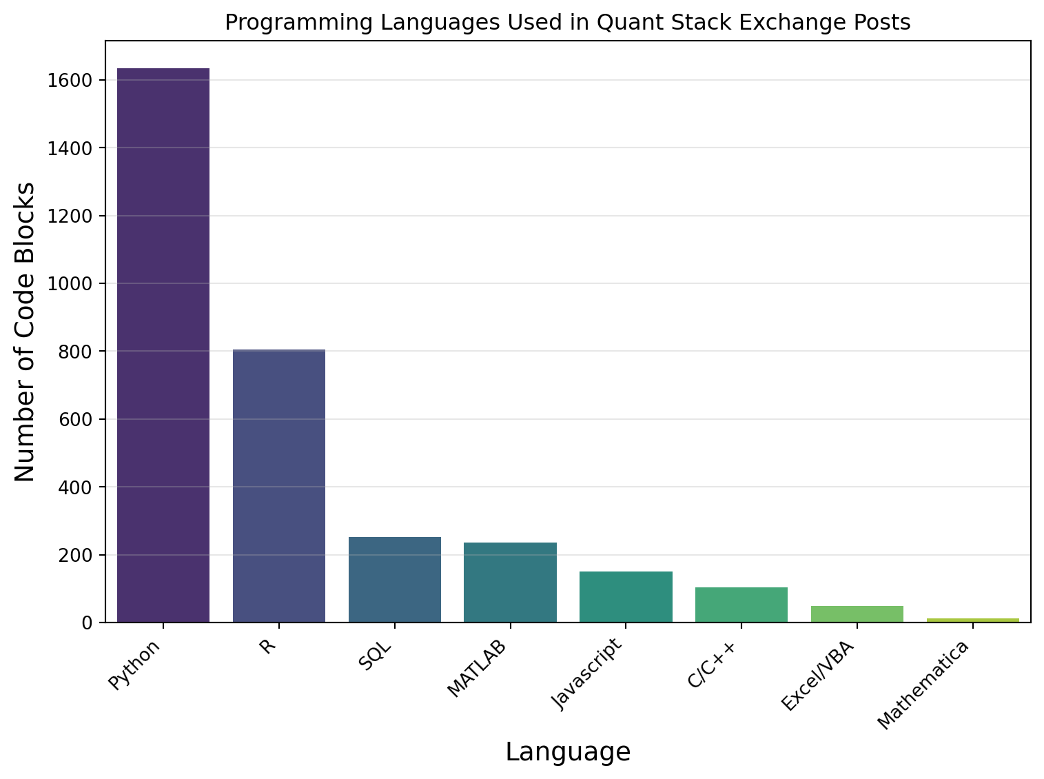
Figure 5 shows a bar chart of the distribution of programming languages in posts on the Quant Stack Exchange site. For plot, the ‘Unknow’, ‘Markdown/HTML’, ‘Formula’, ‘Latex’, and ‘Mathemtical Notation’ categories were removed to focus on actual languages used in software programming. From the figure, it is observed that Python is twice as popular as R, eight times more popular than SQL or MATLAB, and approximately sixteen times more popular than Javascript or C/C++.

# Programming Language Distribution
plt.figure(figsize=(8, 6))

# Filter for languages with >10 occurrences and not the unknown, markdown,
#  formula, notation or latex categories
language_counts = language_counts.loc[(~language_counts.index.str.contains(
    "Unk|Mark|Form|not|latex")) & (language_counts > 10)] 

sns.barplot(x=language_counts.index, y=language_counts.values,
 palette="viridis")
plt.xlabel("Language", fontsize=14)
plt.ylabel("Number of Code Blocks", fontsize=14)
plt.xticks(rotation=45, ha="right")
plt.grid(axis="y", alpha=0.3)
plt.title("Programming Languages Used in Quant Stack Exchange Posts")
plt.tight_layout()
plt.show()

Figure 5: Programming Languages Used in Quant Stack Exchange Posts

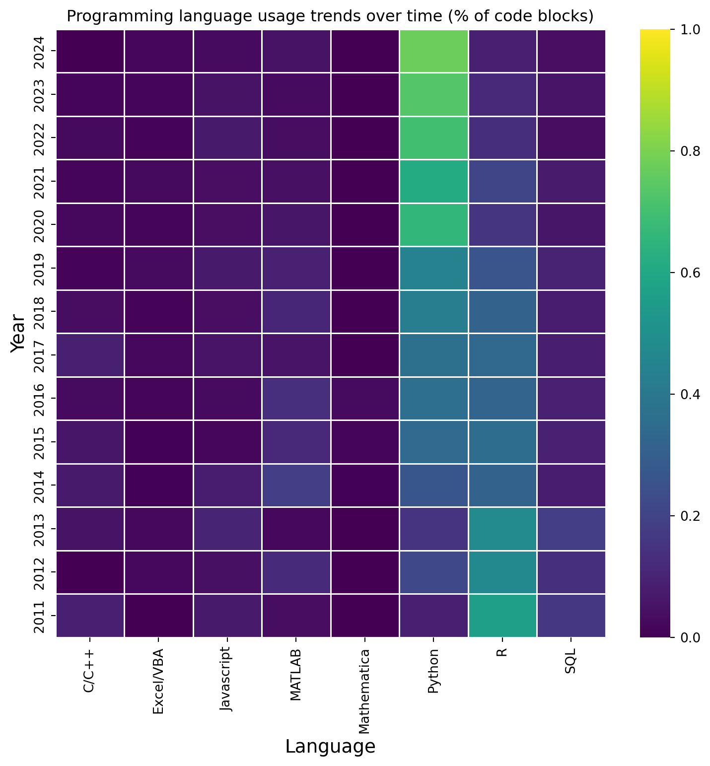
Language Usage Over Time

Based on all the posts, Python may be the most popular programming language, but has it always been the most popular? A heatmap of language usage over time was created to answer this question. The creation data of posts was used to create a column of the year of the posts in the posts_with_code data frame. The language data was joined with the post dates using an inner join on ‘PostId’ from the language data frame and the ‘Id’ from the post dates data frame. The languages were then filtered to remove the ‘Unknow’, ‘Markdown/HTML’, ‘Formula’, ‘Latex’, and ‘Mathemtical Notation’ categories. A cross-table was created using the ‘Year’ and ‘Language’, and the number of code blocks per year was calculated by performing a sum on the table columns. The data in cross-table were then normalised using the count per year. Leaving the data as a percentage of code blocks for that year. This was done because the number of code blocks per year increased with time, and we are only interested in the change in the percentage of a language used for a given year.

# Add year column using creationDate
posts_with_code["Year"] = posts_with_code["CreationDate"].dt.year
    
# Join language data with post dates
language_dates = pd.merge(code_df, posts_with_code[["Id", "Year", "CodeCount"]],
  left_on="PostId", right_on="Id")
language_dates = language_dates[~language_dates["Language"].str.contains(
    "Unk|Mark|Form|Not|Latex")]

# Count languages by year
language_by_year = pd.crosstab(
    language_dates["Year"], language_dates["Language"])

# Count the number of code blocks per year
code_blocks_by_year = language_by_year.sum(axis=1)

language_by_year_norm = language_by_year.div(code_blocks_by_year, axis="index")

Figure 6 shows the evolution of the usage of each programming language between 2011 and 2024. Most notable in the figure is the rise of Python and the demise of R. R was the most popular language from 2011 until 2015. In 2015 Python and R had similar popularity; however, in 2020, Python became the dominant language used in the code blocks of the site, wih approximately 80% of the detected languages usage being Python. Another interesting feature is that SQL usage has declined since 2014. It is unlikely that people have stopped using databases, but more likely that people are now using Python to interact with databases rather than SQL. All other programming languages follow a similar trend to SQL; their usage was highest around 2011 but has dropped since 2017.

plt.figure(figsize=(8, 8))

ax = sns.heatmap(language_by_year_norm, vmin=0, vmax=1, annot=False,
 linewidth=0.5, cmap="viridis", fmt=".2f")
plt.ylabel("Year", fontsize=14)
plt.xlabel("Language", fontsize=14)
ax.invert_yaxis()
plt.tight_layout()
plt.title("Programming language usage trends over time (% of code blocks)")
plt.show()

Figure 6: Programming language usage trends over time (% of code blocks)

Time taken for a question to be answered

If I were to post a question today, how long would I need to wait until someone answered it? This question is the focus of this section.

Data preparation

The response time of answering a post needs to be calculated; this is done by creating two data frames from the post data frame, one containing the questions (PostTypeId=1) and the other containing the answers (PostTypeId=2). These two data frames are then merged using an inner joint on ‘Id’ from the questions and ‘ParentId’ from the answers, with the result being stored in a data frame called answered_df. Columns with the same name in each data frame are kept using the suffixes _question and _answer. The time in minutes to answer a question is calculated from the difference in creation dates. Answers that are faster than one minute are not likely to be correct and, therefore, are excluded from the data. Since there can be multiple answers to a question, we take the fastest answer response using group by and the min() function.

# Response time calculation
questions_df = posts[posts["PostTypeId"]==1].copy()
answers_df = posts[posts["PostTypeId"]==2].copy()

# Merge questions with their answers
aswered_df = pd.merge(
    questions_df[["Id", "CreationDate"]],
    answers_df[["ParentId", "CreationDate"]],
    left_on="Id",
    right_on="ParentId",
    suffixes=("_question", "_answer")
)
    
# Calculate time difference in minutes
aswered_df["TimeInterval"] = (
    (aswered_df["CreationDate_answer"] - aswered_df["CreationDate_question"])
    .dt.total_seconds() / 60
)

# Drop times less than 1 minute
aswered_df = aswered_df[~(aswered_df["TimeInterval"] < 1) ]

# Group by question Id and find the minimum time interval
response_df = aswered_df.groupby("Id")["TimeInterval"].min().reset_index()
    
# Sort by question Id
response_df = response_df.sort_values("Id")

Distribution of answer response time

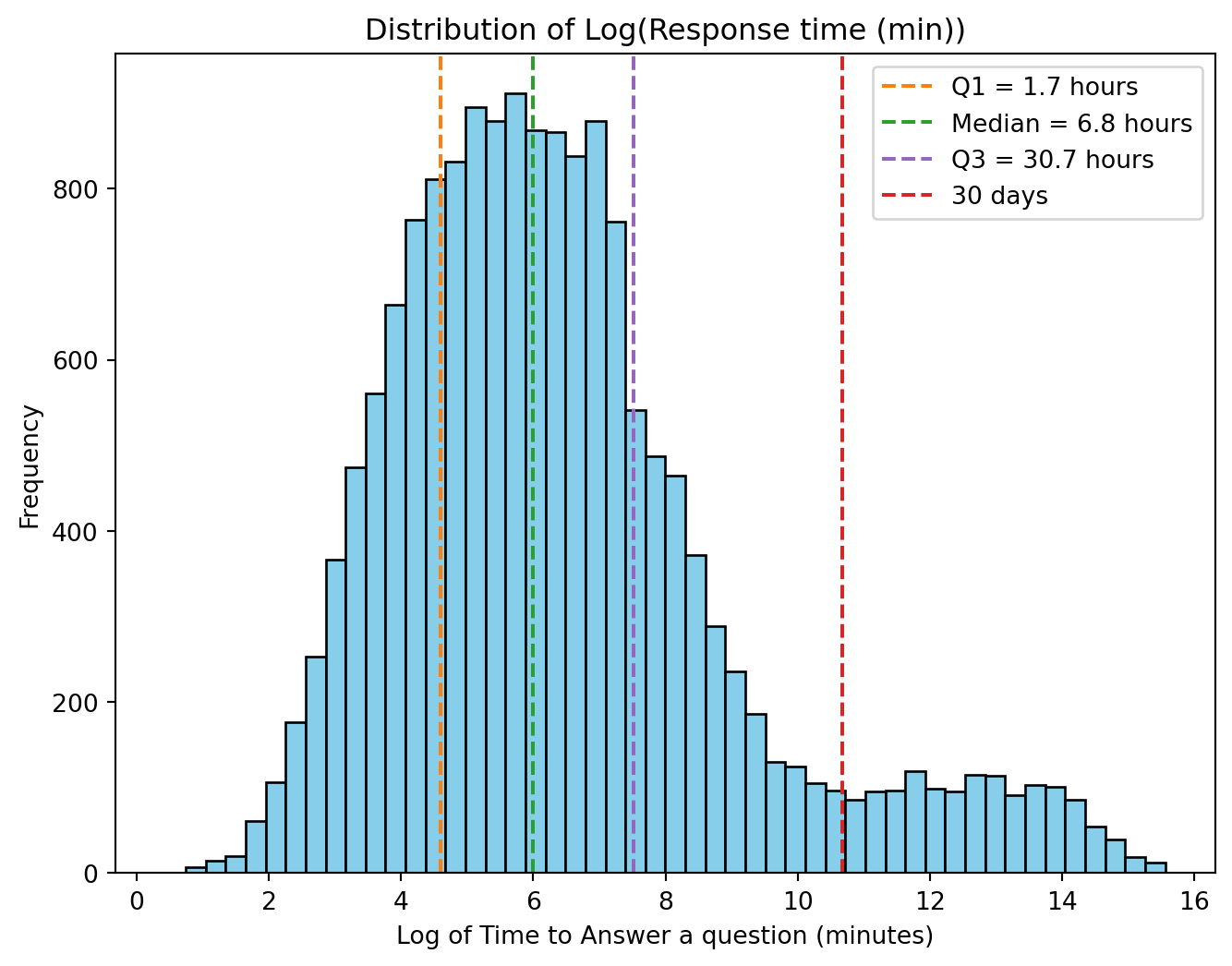
Figure 7 shows the distribution of the log of the time taken in minutes to answer a question. Several vertical lines have been added to the figure to show the first quartile, the median, the third quartile and a 30-day response time. The distribution is bimodal, with the peak of the primary mode around 6.8 hours and the secondary peak around 307 days. What factors would influence the second mode in the distribution?

The Quant Stack Exchange site is a community-driven Q&A website governed by a reputation system. It rewards the users by giving repuation points and badges for the usefulness of their posts. The response time to answer a question depends on a number of factors, such as the question’s quality and complexity, the availability of experts and the experts’ interest in the question topic. For this study, only the relationship between the complexity of the question and the response time to answer is considered.

# Create histogram
plt.hist(np.log(response_df["TimeInterval"]), bins=50, color="skyblue",
 edgecolor="black")

# Add a vertical line at Q1
plt.axvline(x=4.6, color="tab:orange", linestyle="--", label="Q1 = 1.7 hours")

# Add a vertical line at 1 days
plt.axvline(x=6, color="tab:green", linestyle="--", label="Median = 6.8 hours")

# Add a vertical line at Q1
plt.axvline(x=7.51, color="tab:purple", linestyle="--", label="Q3 = 30.7 hours")

# Add a vertical line at 30 days
plt.axvline(x=10.67, color="tab:red", linestyle="--", label="30 days")

plt.xlabel("Log of Time to Answer a question (minutes)")
plt.ylabel("Frequency")
plt.legend()
plt.title("Distribution of Log(Response time (min))")
plt.show()

Figure 7: Distribution of the log of the time in minutes to answer a question

Relationship between response time and question complexity

To investigate the association between question complexity and the time taken to answer the question, the following parameters were studied:

• The density of the mathematics in the question
• The length of the question
• Repuation of the asker
• Readability of the question

I define the density of mathematics in a question as the number of Latex equation patterns per word in the question after code blocks have been removed. A function was created to calculate the density of the mathematics used in a question. The function takes the body of a post, finds code blocks using a regex, and replaces them with an empty string; then, Latex math patterns are found using regex, and the number is counted. The post’s word count is calculated by finding all the words in the posts using a regular expression. The density is the number of Latex math expressions divided by the word count.

# Function to calculate math density using regex
def calculate_math_density(body):
    """
    Calculate math density from post body using various regex patterns.

    :param body: string of the body text
    :return: Float containg the density of math in the post body
    """
    if pd.isna(body):
        return []
    
    body = body.lower()
    
    # Remove code blocks
    code_pattern = re.compile(r"<code>(.*?)</code>", re.DOTALL)
    body = re.sub(code_pattern, "", body)

    math = []
    
    # Find inline LaTeX math (between $ signs)
    inline_pattern = re.compile(r"\$([^$]+)\$")
    inline_math = inline_pattern.findall(body)
    math.extend(inline_math)
    
    # Find display LaTeX formulas (between $$ signs)
    display_pattern = re.compile(r"\$\$([^$]+)\$\$")
    display_math = display_pattern.findall(body)
    math.extend(display_math)
    
    # Count words (simple split)
    num_words = len(re.findall(r"\w+", body))

    # Avoid division by zero
    if num_words == 0:
        return 0

    # Density = math matches per word
    return len(math) / num_words

After the mathematics density is calculated for each question, a left join is performed between the response time and the question data frames to get the response time for each question with an answer. This is stored in a new questions_response_df data frame. The cleaned posts data frame created in Section 4.3 is also merged with the question data to leave only rows in the clean posts data frame that are in the questions data. The tag type information in the cleaned posts data frame will be used to colour the points in the following scatter plots.

# Apply math density calculation to posts
questions_df["MathDensity"] = questions_df["Body"].apply(calculate_math_density)

# Merge response_df with questions to get response time for questions with
#  an answer
question_response_df = pd.merge(
    response_df,
    questions_df,
    on="Id",
    how="left"
)

# Merge to ensure the rows are the same. 
posts_cleaned_filtered = posts_cleaned.merge(
    question_response_df[["Id"]], on="Id", how="inner")

# Plot Response time versus mathematical density
palette = ["tab:red", "tab:green"]

plt.figure(figsize=(10, 6))
scatter = sns.scatterplot(x=question_response_df["MathDensity"],
    y=np.log(question_response_df["TimeInterval"]),
    alpha=0.6,hue=posts_cleaned_filtered["TagType"], palette=palette)

plt.xlabel("Mathematical density")
plt.ylabel("Log(Response time (min))")
plt.title("Scatter Plot of Log(Response time (min)) vs. Mathematical density")
plt.show()

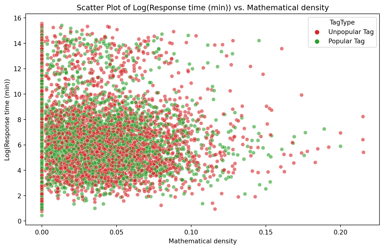
Figure 8: Scatter plot of Log(Response time (min)) vs. Mathematical density

sp_correlation_md = round(question_response_df["MathDensity"].corr(
    np.log(question_response_df["TimeInterval"]), method="spearman"),3)
print(f"""The Spearman correlation between Mathematical density and """
"""Log(Response time) is {sp_correlation_md:.3f}""")

The Spearman correlation between Mathematical density and Log(Response time) is {sp_correlation_md:.3f}

Figure 8 shows a scatter plot between Log(Response time) and Mathematical density with the points coloured by tag type. The first notable feature of this plot is that there are no tags of type ‘No Tag’. This shows that all answered questions had at least one tag set. The distribution of ‘Unpopular’ and ‘Popular’ tags is random and scattered throughout the plots with no visible clustering. The second notable feature is that there are a lot of answered questions that have no mathematics in them, i.e., a math density of zero. Lastly, the high response time is visible for all mathematical density values. The Spearman correlation coefficient (-0.004) shows no consistent monotonic relationship between the Log(Response time) and the Mathematical density.

# Plot Log response versus Log post length
plt.figure(figsize=(10, 6))
scatter = sns.scatterplot(x=np.log(question_response_df["Body"].apply(len)),
    y= np.log(question_response_df["TimeInterval"]),
    alpha=0.6,hue=posts_cleaned_filtered["TagType"], palette=palette)

plt.xlabel("Log(Post length (characters))")
plt.ylabel("Log(Response time (min))")
plt.title(
"Scatter plot of Log(Response time (min)) vs. Log(Post length (characters))")
plt.show()

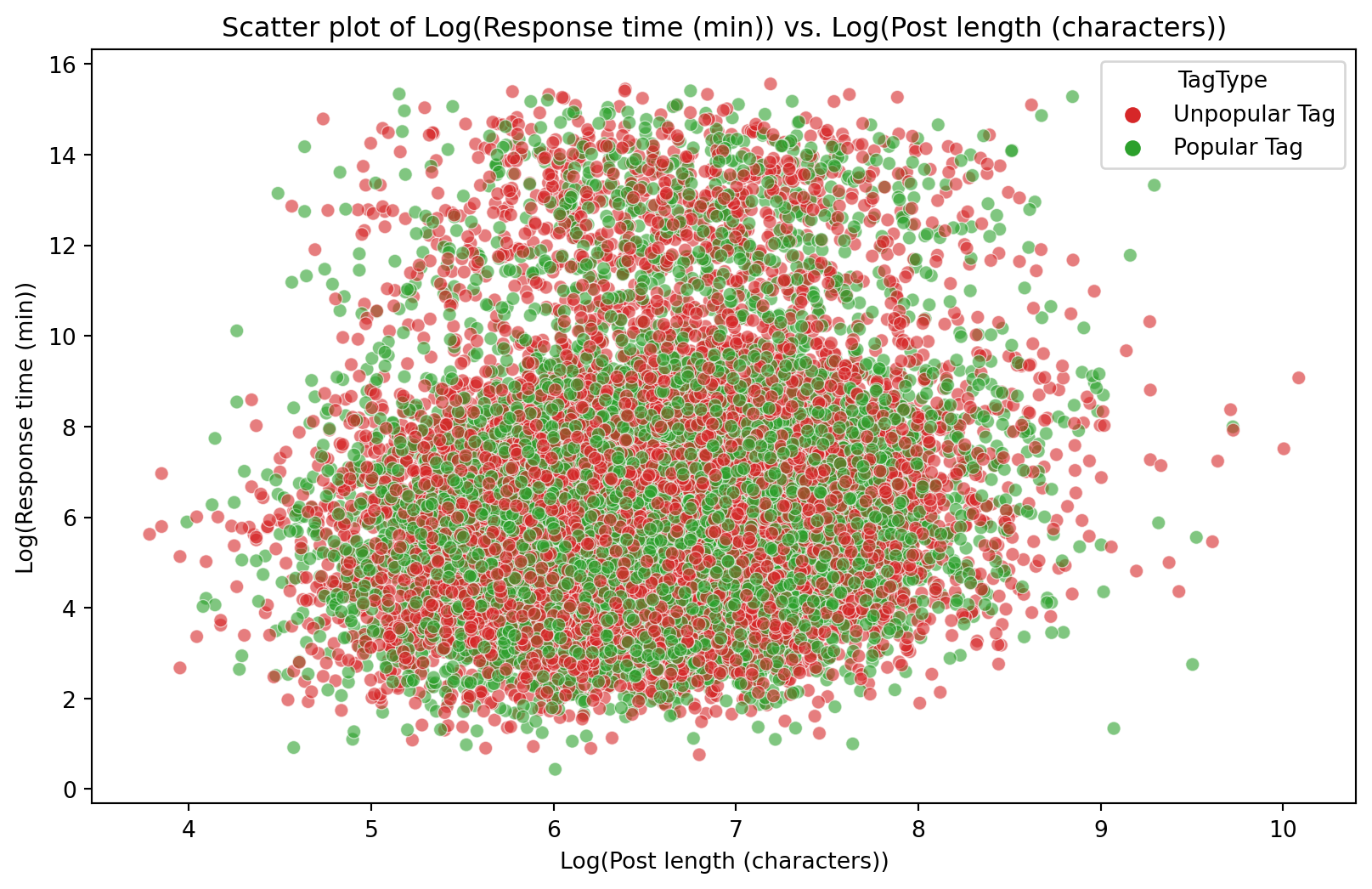
Figure 9: Scatter plot of Log(Response time (min)) vs. Log(Post length (characters))

sp_correlation_pl = round(np.log(question_response_df['Body'].apply(len)).corr(
    np.log(question_response_df['TimeInterval']), method='spearman'), 3)
print(f"""The Spearman correlation between Log(Post length) and """
"""Log(Response time) is {sp_correlation_pl:.3f}""")

The Spearman correlation between Log(Post length) and Log(Response time) is {sp_correlation_pl:.3f}

Figure 9 shows a scatter plot between Log(Response time) and Log(Post length). The majority of answered questions had a length between 150 and 3000 characters. Again, the distribution of the tag type is random and spreads throughout the entire domain of the plot. Two clusters are visible, one with a high response time and the other with a lower response time. The Spearman correlation coefficient (0.143) shows no consistent monotonic relationship between the Log(Response time) and Log(Post length).

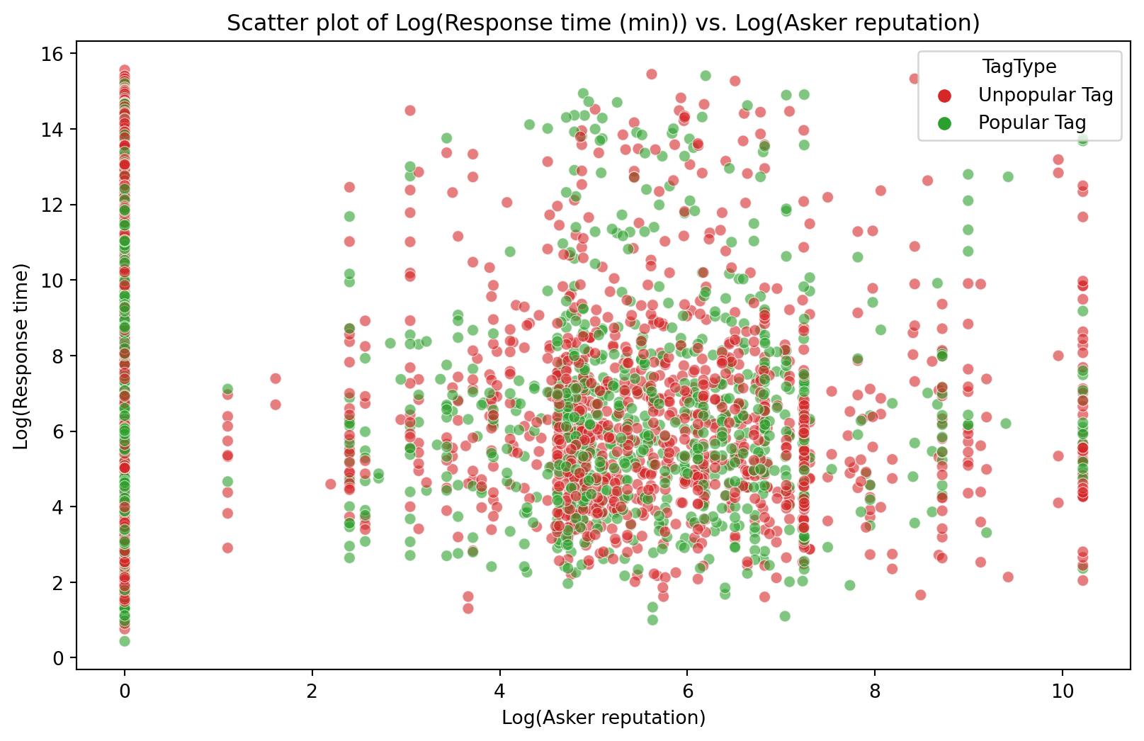
questions_reputation_df = pd.merge(question_response_df, 
    users[['Id', 'Reputation']], left_on='OwnerUserId', right_on='Id',
    how='left')
questions_reputation_df['Reputation'].fillna(1, inplace=True)

plt.figure(figsize=(10, 6))
scatter = sns.scatterplot(
    x=np.log(questions_reputation_df['Reputation']),
    y=np.log(questions_reputation_df['TimeInterval']),
    alpha=0.6,hue=posts_cleaned_filtered['TagType'], palette=palette)

plt.xlabel('Log(Asker reputation)')
plt.ylabel('Log(Response time)')
plt.title('Scatter plot of Log(Response time (min)) vs. Log(Asker reputation)')
plt.show()

C:\Users\darrin\AppData\Local\Temp\ipykernel_21820\578517144.py:4: FutureWarning:

A value is trying to be set on a copy of a DataFrame or Series through chained assignment using an inplace method.
The behavior will change in pandas 3.0. This inplace method will never work because the intermediate object on which we are setting values always behaves as a copy.

For example, when doing 'df[col].method(value, inplace=True)', try using 'df.method({col: value}, inplace=True)' or df[col] = df[col].method(value) instead, to perform the operation inplace on the original object.

Figure 10: Scatter plot of Log(Response time (min)) vs. Log(Asker reputation)

sp_correlation_ar = round(np.log(questions_reputation_df['Reputation']).corr(
    np.log(question_response_df['TimeInterval']), method='spearman'), 3)
print(f"""The Spearman correlation between Log(Askers reputation) and """
"""Log(Response time) is {sp_correlation_ar:.3f}""")

The Spearman correlation between Log(Askers reputation) and Log(Response time) is {sp_correlation_ar:.3f}

Figure 10 shows a scatter plot between Log(Response time) and Log(Asker reputation). Many users have a low reputation of one, and a scattering of users with a high reputation ask questions. The tag type again shows a random distribution throughout the plot. Questions from users with high reputations can also take a long time to answer. Again, the Spearman correlation coefficient (0.143) shows no consistent monotonic relationship between the Log(Response time) and Log(Askers reputation).

# Function to clean text
def clean_body(text):
    """
    Removes number, html blocks and latex code from a given string.

    :param text: String to clean
    :return: clened text
    """
    if pd.isna(text):
        return ""
    
    # Remove numbers
    text = re.sub(r"\d+", "", text)

    # Remove inline math $...$
    text = re.sub(r"\$.*?\$", "", text)
    
    # Remove display math $$...$$
    text = re.sub(r"\$\$.*?\$\$", "", text)

    # Remove <code> </code> blocks
    code_pattern = re.compile(r"<code>(.*?)</code>", re.DOTALL)
    text = re.sub(code_pattern, "", text)
    
    return text

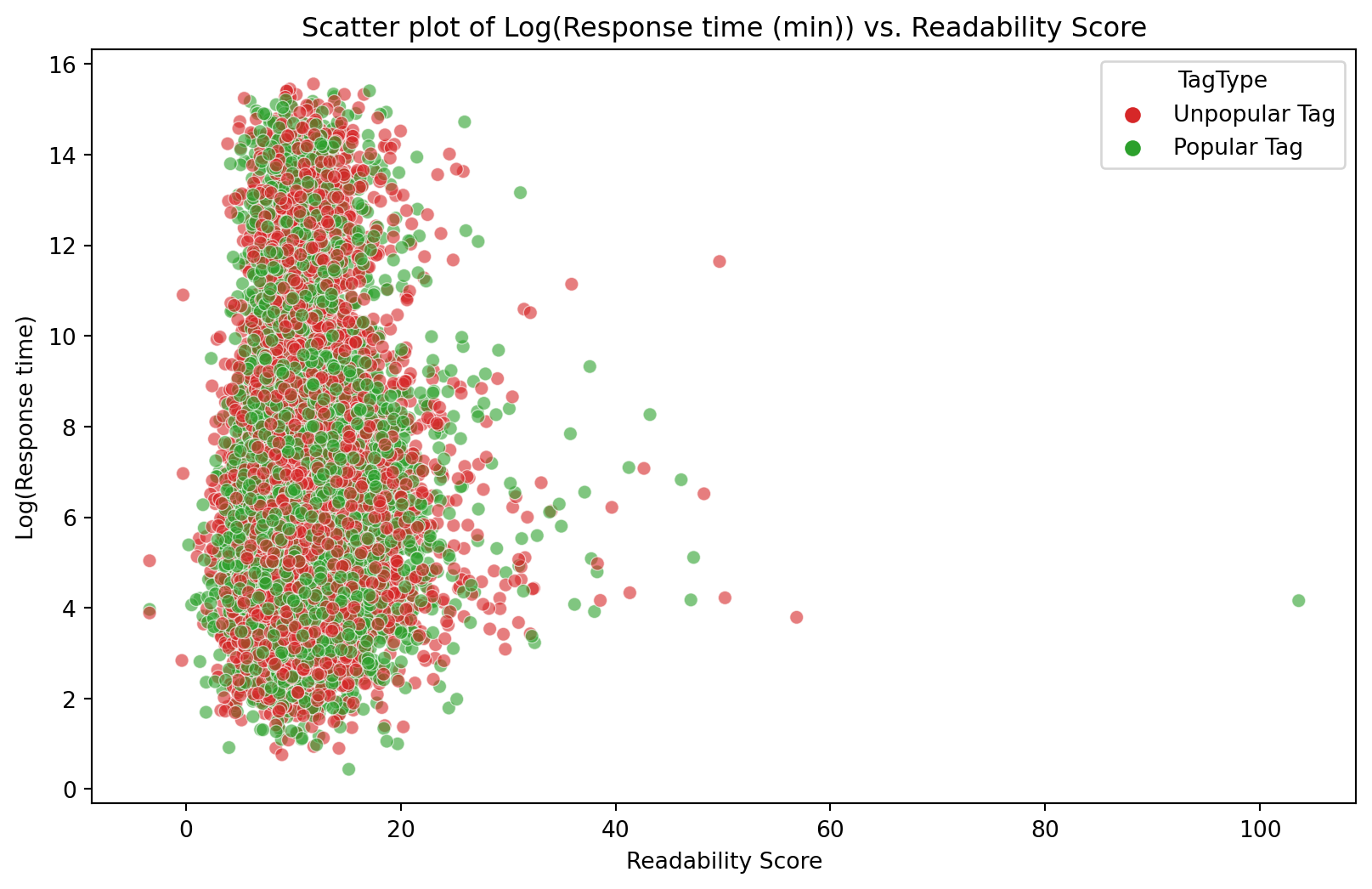
# Clean html and Latex from body
question_response_df["CleanedBody"] =  question_response_df["Body"].apply(
    clean_body)

#Calculating readability score using Flesch Kincaid Grade
question_response_df["FleschKincaidGrade"] =  question_response_df["CleanedBody"
    ].apply(textstat.flesch_kincaid_grade)

plt.figure(figsize=(10, 6))
scatter = sns.scatterplot(
    x=question_response_df["FleschKincaidGrade"],
    y=np.log(question_response_df["TimeInterval"]),
    alpha=0.6,hue=posts_cleaned_filtered["TagType"], palette=palette)

plt.xlabel("Readability Score")
plt.ylabel("Log(Response time)")
plt.title("Scatter plot of Log(Response time (min)) vs. Readability Score")
plt.show()

Figure 11: Scatter plot of Log(Response time (min)) vs. Log(Asker reputation)

sp_correlation_read = round(question_response_df["FleschKincaidGrade"].corr(
    question_response_df["TimeInterval"], method="spearman"), 3)
print(f"""The Spearman correlation between asker's reputation and response """
"""time is {sp_correlation_read:.3f}""")

The Spearman correlation between asker's reputation and response time is {sp_correlation_read:.3f}

The readability score of a question was calculated using the Flesch Kincaid Grade. Higher numbers indicate harder-to-read posts. The readability score was calculated on the posts’s body text after the mathmatical formula and code blocks were removed. Figure 11 shows a scatter plot between the Log(Response time) and Readability score. Most questions have a readability score of around 13, with some scoring above 20. There is no visible trend between response time and readability score. The Spearman correlation coefficient (0.074) shows no consistent monotonic relationship between the Log(Response time) and Readability score.

It has been seen that there is no consistent monotonic relationship between Log(Response time) and either of Mathematical density, Log(Post length), Log(Asker reputation) or Readability score. The non-existence of a relationship between the Log(Response time) and the other variables does not mean we can rule out any relationship between these variables as there could still be:

• Multivariate relationships where variables might only show associations in combination
• Interaction effects among the independent variables

Further analysis that is beyond the scope of this work would be needed to draw a conclusion about the impact of question complexity on the time it takes to be answered.

Summary

Analysis of the Quant Stack Exchange site has been performed for the geographic distribution of the site’s users, the popular words used in posts, the popularity of tags used in posts, the type of programming language discussed, and how this has changed over the site’s life, and the response time to answering questions, and the relationship to question complexity.

User Geographic Distribution

• Users are heavily concentrated in Europe, US coasts, and India
• Lower representation in Africa, South America, and Southeast Asia
• Australian users mainly in capital cities (except Perth)

Popular Content Analysis

• The most common words in the top questions: “option,” “volatility,” and “model”.
• Financial terminology dominates high-scoring questions
• Top tags evolved from 2011 to 2024: options, options pricing, and Black-Scholes consistently popular
• Programming tags gained popularity, especially during COVID-19

Cross-Site References

• ~10% of posts contain website links (average four links per post)
• 84% of links are to external sites, with academic resources being common
• 16% link to other Stack Exchange/Overflow sites
• Images account for 43% of all post links

Programming Language Trends

• Python overtook R as the dominant language (80% of code blocks by 2020)
• R was most popular from 2011-2015
• SQL and other languages have declined since 2017
• About 10% of posts contain code blocks

Question Response Time Analysis

• Distribution is bimodal: peaks at ~6.8 hours and ~307 days
• No strong correlation was found between response time and:
  • Mathematical content density
  • Post length
  • Asker reputation
  • Text readability

The analysis suggests that while the site has evolved, particularly in programming language preferences, the factors that determine how quickly questions receive answers remain complex and possibly involve multivariate relationships beyond the scope of this analysis.