description = 'Darrin William Stephens, SIT741: Statistical Data Analysis, Task T03.P3'Distributions
Introduction
In this task, the “fitdistrplus” package is used to fit distributions to weather data for New York city airports and compare the goodness of fit.
Task steps
1. Define a string and print it
This section defines a string containing my name, the unit name and the task name.
Print the string using the cat() function.
cat(description)Darrin William Stephens, SIT741: Statistical Data Analysis, Task T03.P32. Read the dataset
The weather data in the “nycflights13” dataset was downloaded as a CSV file from https://github.com/tidyverse/nycflights13/blob/main/data-raw/weather.csv. The weather data can then be loaded into R.
weather_data = read.csv('weather.csv')3. Print variable names/types and select data for next steps.
Create a tibble containing the names and data types for each variable. The sapply() function can be used to get the type of each variable.
names_types = tibble(Variable_Name = names(weather_data), Type = sapply(weather_data, class))
print(names_types)
# A tibble: 15 × 2
Variable_Name Type
<chr> <chr>
1 origin character
2 year integer
3 month integer
4 day integer
5 hour integer
6 temp numeric
7 dewp numeric
8 humid numeric
9 wind_dir integer
10 wind_speed numeric
11 wind_gust numeric
12 precip numeric
13 pressure numeric
14 visib numeric
15 time_hour characterFor the next tasks, I selected the wind_speed and pressure variables and filtered out any null values.
4. Histograms and Q-Q plots
Wind Speed
The histogram and Q-Q plots for the wind speed are shown below. An outlier in the data stretches the scale of the horizontal axis in the histogram, making the distribution hard to see. An outlier is visible in the Q-Q plot in the top right-hand corner of the plot.
# Histogram plot
reduced_data |>
  ggplot(aes(x = wind_speed)) +
  geom_histogram(binwidth = 2.2, fill ="skyblue", color = "black") +
  labs(
    title = "Distribution of Wind Speed",
    x = "Wind Speed (mph)",
    y = "Frequency"
  ) +
  theme(plot.title = element_text(hjust = 0.5))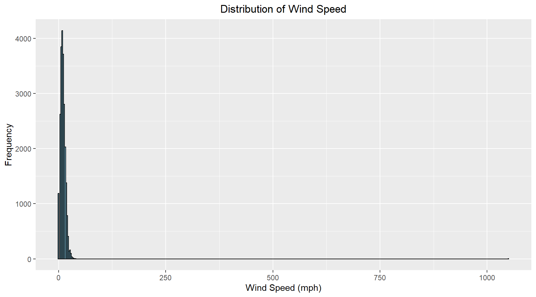
# Q-Q plot
reduced_data |>
  ggplot(aes(sample = wind_speed)) +
  geom_qq() +
  labs(
    title = "Q-Q plot for Wind Speed",
  ) +
  theme(plot.title = element_text(hjust = 0.5))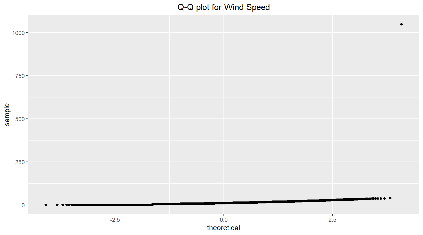
The outlier identified in the wind speed data can be removed by selecting data that is between +- 1.5*IQR from the mean. The histogram and Q-Q plot for the wind speed without the outlier are shown below.
reduced_data_clean |>
  # Remove any null values before plotting
  ggplot(aes(x = wind_speed)) +
  geom_histogram(binwidth=2.2, fill ="skyblue", color = "black") +
  labs(
    title = "Distribution of Wind Speed without outlier",
    x = "Wind Speed (mph)",
    y = "Frequency"
  ) +
  theme(plot.title = element_text(hjust = 0.5))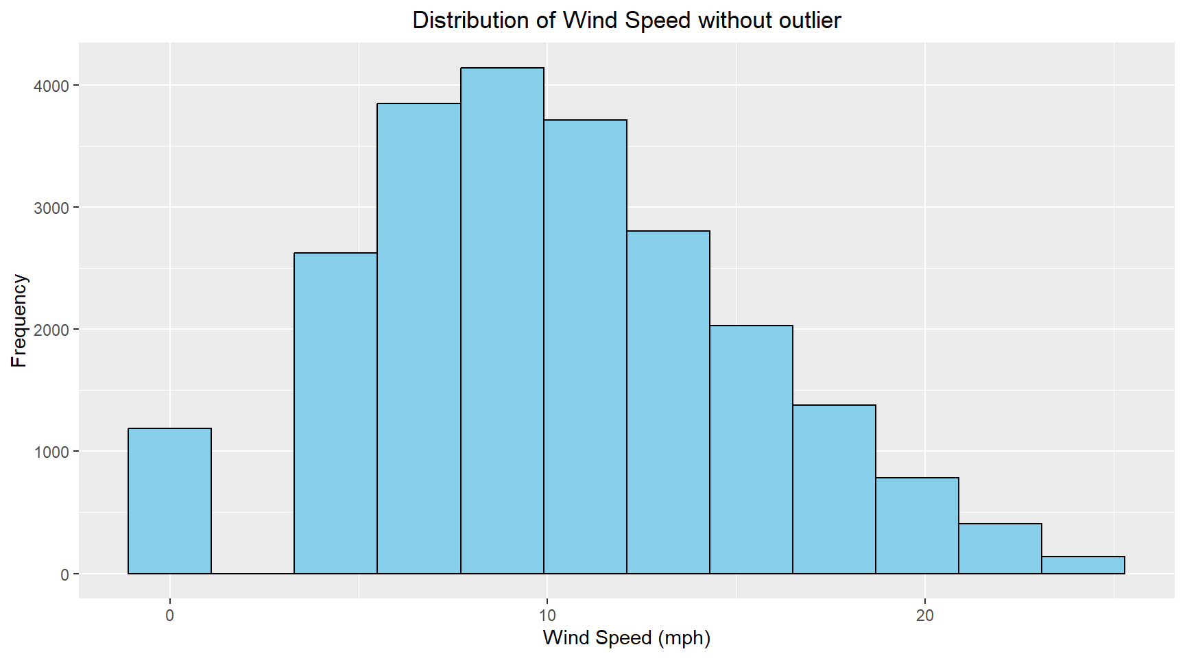
# Q-Q plot
reduced_data_clean |>
  ggplot(aes(sample = wind_speed)) +
  geom_qq() +
  labs(
    title = "Q-Q plot for Wind Speed without outlier",
  ) +
  theme(plot.title = element_text(hjust = 0.5))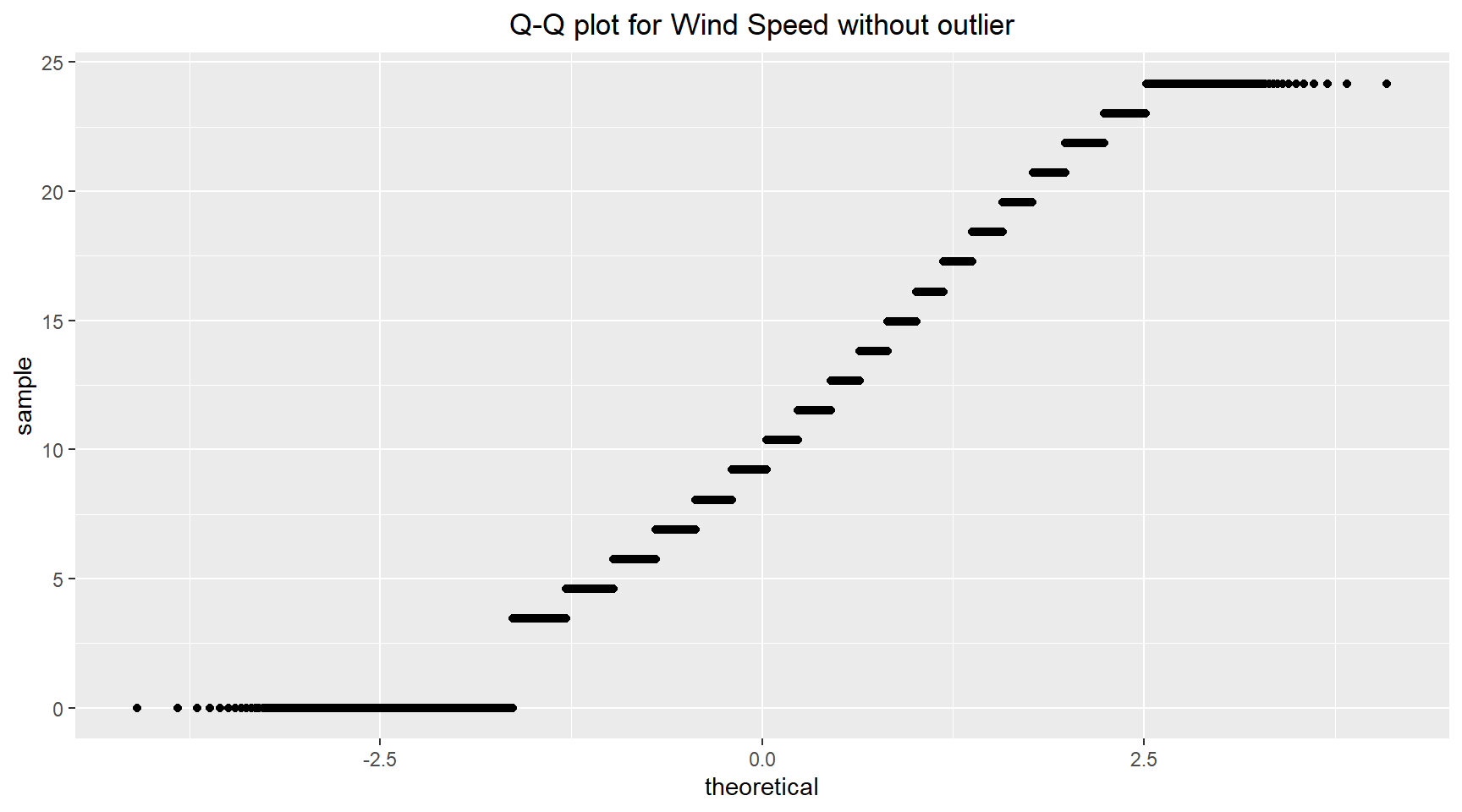
Pressure
The histogram and Q-Q plots for the pressure are shown below. The histogram shows signs of some outliers on the left side (lower pressures) of the distribtuion. To confirm the prescence of outliers, I created a box plot. The boxplot shows outliers at on both side of the distribution.
reduced_data_clean |>
  ggplot(aes(x = pressure)) +
  geom_histogram(binwidth = 3, fill = "forestgreen", color = "black") +
  labs(
    title = "Distribution of Pressure",
    x = "Pressure (millibar)",
    y = "Frequency"
  ) +
  theme(plot.title = element_text(hjust = 0.5))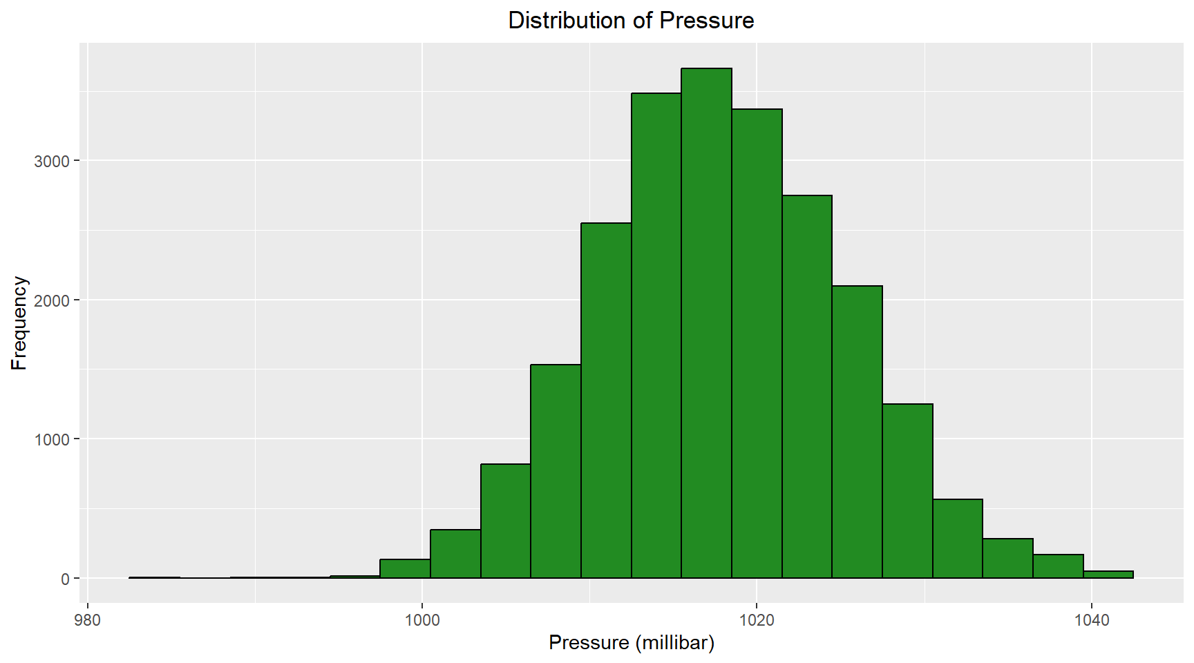
# QQ plot
reduced_data_clean |>
  # Remove any null values before plotting
  filter(!is.na(pressure)) |>
  ggplot(aes(sample = pressure)) +
  geom_qq() +
  labs(
    title = "Q-Q plot for Pressure",
  ) +
  theme(plot.title = element_text(hjust = 0.5))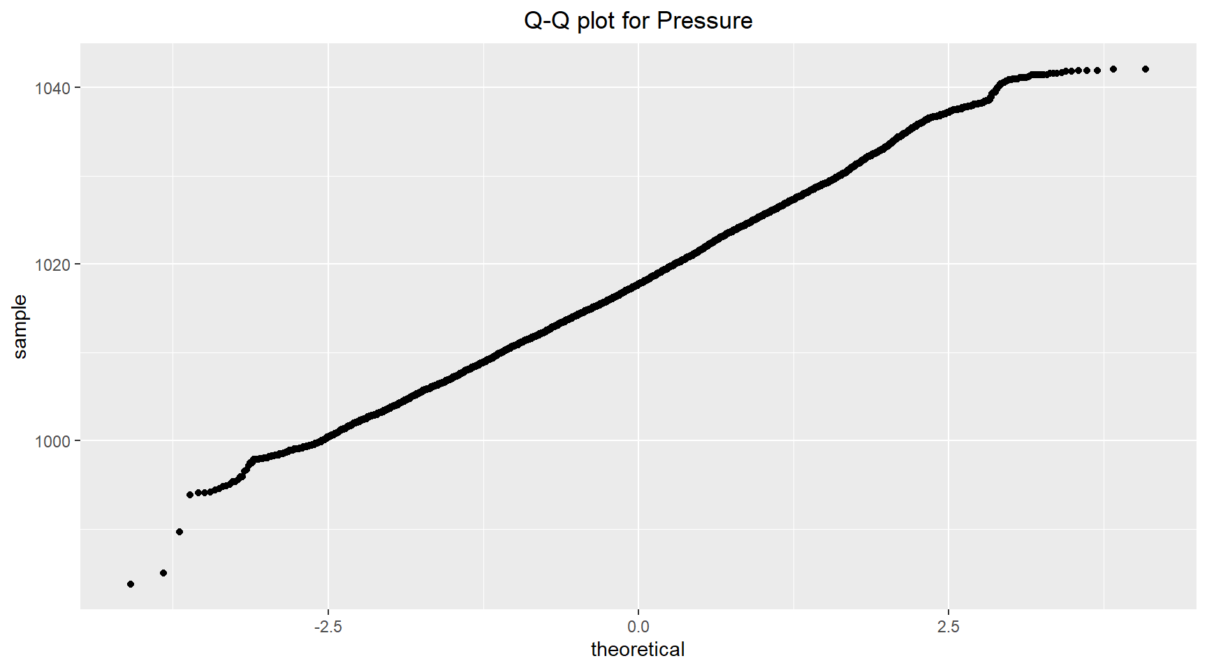
# Boxplot of pressure to confirm existence of outliers.
reduced_data_clean |>
  ggplot(aes(x = "", y = pressure)) +
  geom_boxplot(fill = "orchid", color = "black", outlier.colour = "red", outlier.shape = 1, outlier.size = 4) +
  labs(title = "Pressure",
       x = "",
       y = "Pressure (millibar)") +
  theme(plot.title = element_text(hjust = 0.5))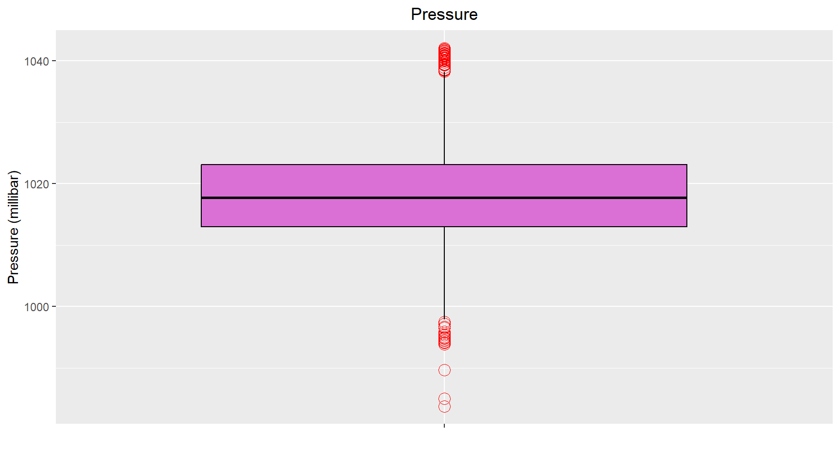
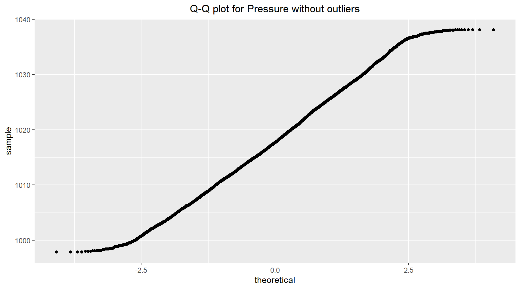
The outliers identified in the pressure data can be removed by selecting data that is between +- 1.5*IQR from the mean. The histogram and Q-Q plot for the pressure without the outliers are shown below.
reduced_data_clean |>
  ggplot(aes(x = pressure)) +
  geom_histogram(binwidth = 3, fill = "forestgreen", color = "black") +
  labs(
    title = "Distribution of Pressure without outliers",
    x = "Pressure (millibar)",
    y = "Frequency"
  ) +
  theme(plot.title = element_text(hjust = 0.5))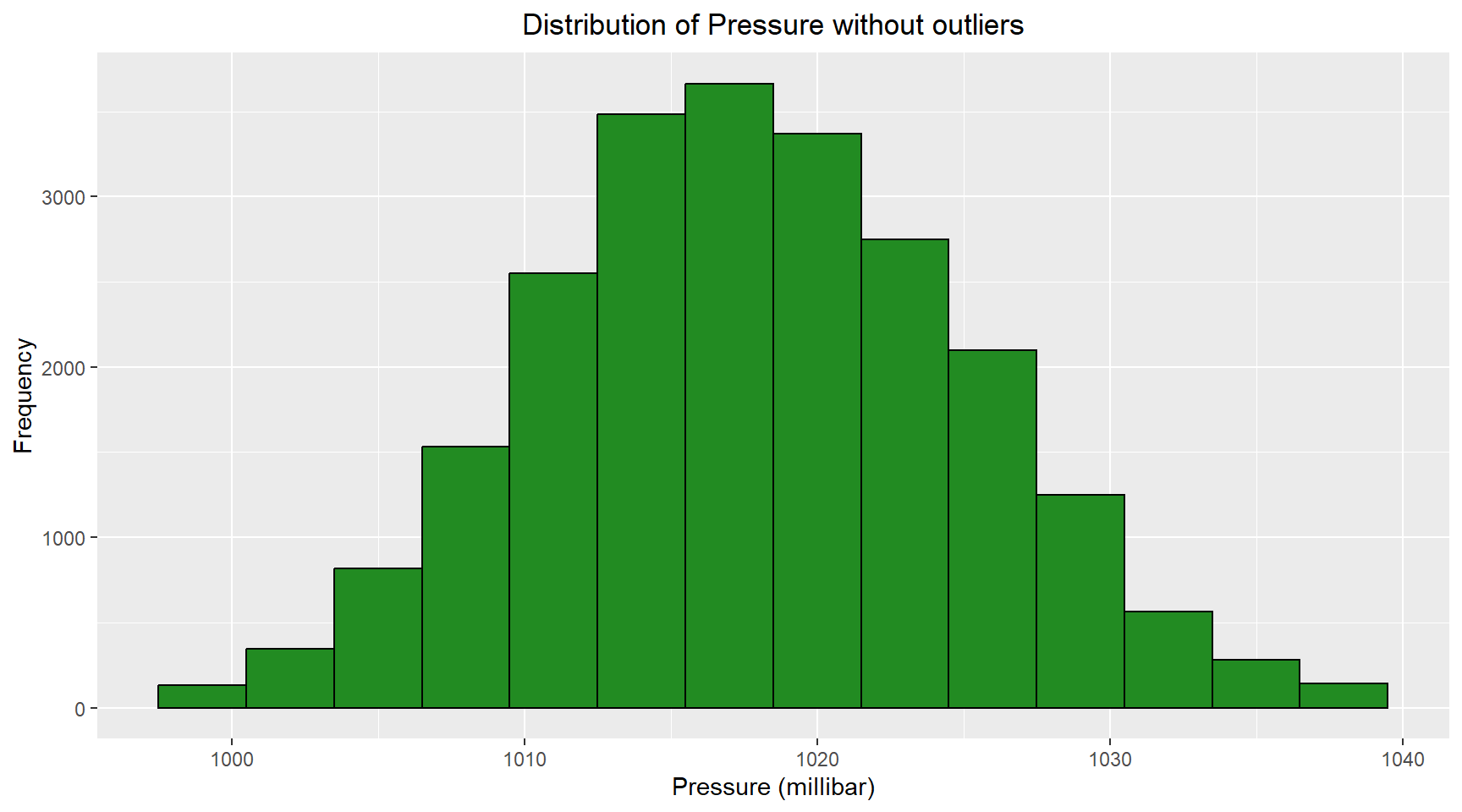
5. Simulated data for Pressure
Before creating simulated data for pressure, I need to determine an appropriate distribution. To determine an appropriate distribution, I created a Cullen and Frey graph as seen below. The estimated kurtosis is 2.76, very close to a normal distribution that has a kurtosis of three. The estimated skewness of 0.099 is small enough to suggest a normal distribution might be appropriate. The suitability of the Normal distribution is is confirmed visually with the proximity of the data point to the Normal distribution point on the Cullen and Frey graph.
descdist(reduced_data_clean$pressure, boot = 100)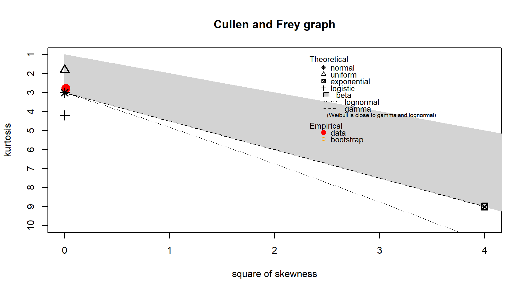
summary statistics
------
min:  997.9   max:  1038.1
median:  1017.7
mean:  1017.949
estimated sd:  7.245498
estimated skewness:  0.09907063
estimated kurtosis:  2.766204
To simulate a normal distribution, I use the rnorm() function with the mean and standard deviation calculated from the existing pressure data. A Cullen and Frey graph is then created for this simulation data. Visually, the only noticeable difference between the Cullen and Frey graphs for the original and simulated pressure is the kurtosis for the simulated data is closer to three. The estimated skewness for the simulated pressure is close to zero compared to the 0.099 for the original pressure. This result isn’t surprising since a normal distribution has a skewness of zero and kurtosis of three.
set.seed(1000)

simulated_data <- reduced_data_clean |>
  mutate(
    sim_pressure= rnorm(n = n(),
                        mean = mean(pressure),
                        sd = sd(pressure)))

descdist(simulated_data$sim_pressure, boot = 100)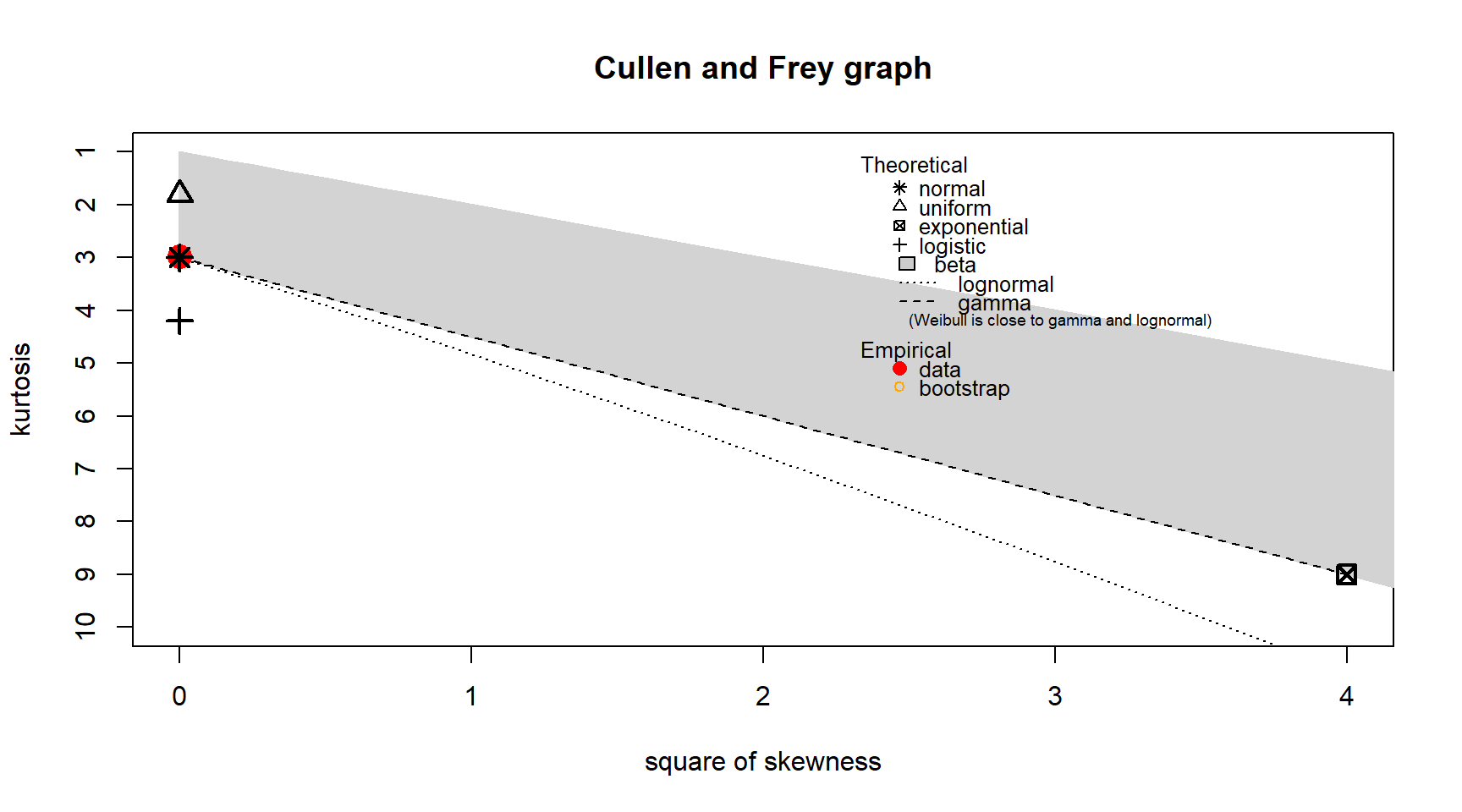
summary statistics
------
min:  984.4058   max:  1049.215
median:  1017.955
mean:  1017.96
estimated sd:  7.193673
estimated skewness:  0.00571225
estimated kurtosis:  2.978431
6. Fitting distributions
Wind Speed
Before fitting a distribution to wind speed, I created a Cullen and Frey graph to identify possible candidate distributions. The wind speed distribution has a kurtosis slightly less than three and a slight positive skewness of 0.294. Several distributions could be suitable, including the Normal, gamma, Weibull, and even log Normal. I know from domain knowledge that a gamma distribution is often used for modelling wind speeds, so I will fit a gamma distribution. The wind speed data contains values at zero. However, the gamma distribution can only have positive values. Therefore, I have chosen to filter out the zero values. These would represent completely still air, which could also be a result of wind speeds below the measurement instrument’s lowest measuring range.
descdist(reduced_data_clean$wind_speed, boot = 100)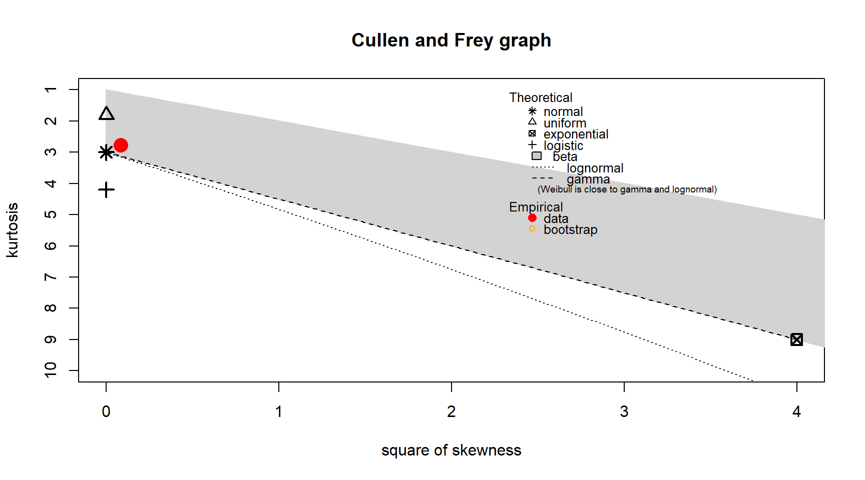
summary statistics
------
min:  0   max:  24.16638
median:  9.20624
mean:  10.09254
estimated sd:  5.184498
estimated skewness:  0.2915728
estimated kurtosis:  2.776651
# Remove the zero wind speeds
reduced_data_clean_removed_zero = reduced_data_clean |>
filter(wind_speed > 0)
# Fit a gamma distribution
fit_ws_G = fitdist(reduced_data_clean_removed_zero$wind_speed, "gamma")
plot(fit_ws_G) 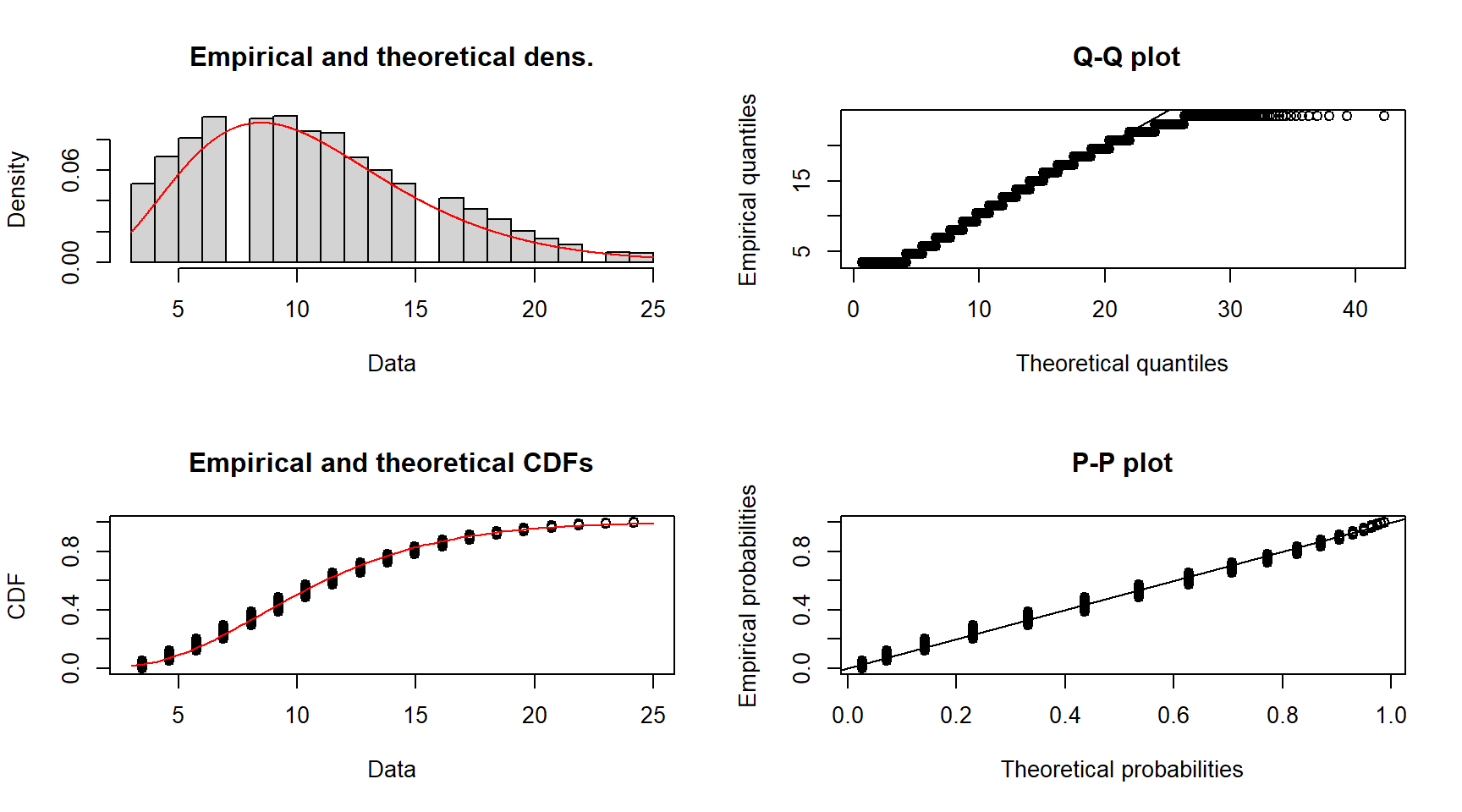
summary(fit_ws_G)Fitting of the distribution ' gamma ' by maximum likelihood
Parameters :
estimate Std. Error
shape 4.8843925 0.045296187
rate 0.4589728 0.004482906
Loglikelihood: -63573.82 AIC: 127151.6 BIC: 127167.6
Correlation matrix:
shape rate
shape 1.0000000 0.9494561
rate 0.9494561 1.0000000Pressure
For the pressure, I have already discussed that it is close to a Normal distribution in step 5. Therefore, I’ll now fit a Normal distribution.
# Fit a Normal distribution
fit_p_N = fitdist(reduced_data_clean$pressure, "norm")

plot(fit_p_N) 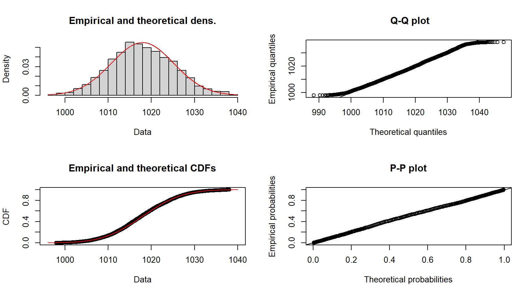
summary(fit_p_N)Fitting of the distribution ' norm ' by maximum likelihood
Parameters :
estimate Std. Error
mean 1017.94946 0.04781075
sd 7.24534 0.03380730
Loglikelihood: -78064.86 AIC: 156133.7 BIC: 156149.8
Correlation matrix:
mean sd
mean 1 0
sd 0 17. Goodness of fit
Visual inspection of the density plot, CDF, Q-Q and P-P plots can be used to assess the goodness of fit. The Q-Q plot emphasises the lack of fit at the distributions tails, while the P-P plot empthasises the lack of fit at the distributions centre. When choosing between multiple distributions, the values of the Aikake’s information criterion (AIC) and Bayesian information criterion (BIC) can be compared. The distribution that gives lower values of these metrics is the better-fitted distribution. An example of this approach is provided for wind speed.
Wind speed
The density and CDF plots for the wind speed show a good fit with both theoretical lines following the data. The P-P plot shows good agreement between the empirical and theoretical probabilities, although some deviation from the theoretical is observed for the lower half of the probabilities. The Q-Q plot shows some deviation at the far left and right of the plot. The deviation is greater at the higher quantiles, suggesting the gamma distribution isn’t fitting well at the tails of the data, especially the right tail.
Example of comparing the fit of multiple distributions. Here, gamma, Normal and log-Normal distributions have been fitted to the wind speed data. Density, CDF, Q-Q, and P-P plots have been produced showing the results for each of the distributions. Visually, it is clear from the density plot that the Normal distribution is the worst fit of the three. We can use the AIC and BIC values to rank the distributions in terms of goodness of fit. The lowest AIC and BIC values indicate the best-fitting distribution. For the wind speed, the gamma distribution is the best fitting, followed by log-normal, and then Normal.
# Fit a normal distribution
fit_ws_N = fitdist(reduced_data_clean_removed_zero$wind_speed, "norm")

# Fit a log-normal distribution
fit_ws_LN = fitdist(reduced_data_clean_removed_zero$wind_speed, "lnorm")

# Combine fits into a list
fits = list(Gamma = fit_ws_G, Normal = fit_ws_N,  LogNormal=fit_ws_LN)

# Create plots
par(mfrow = c(2, 2))
plot.legend <- c("Gamma", "Normal", "Log-Normal")
denscomp(fits, legendtext = plot.legend)
qqcomp(fits, legendtext = plot.legend)
cdfcomp(fits, legendtext = plot.legend)
ppcomp(fits, legendtext = plot.legend)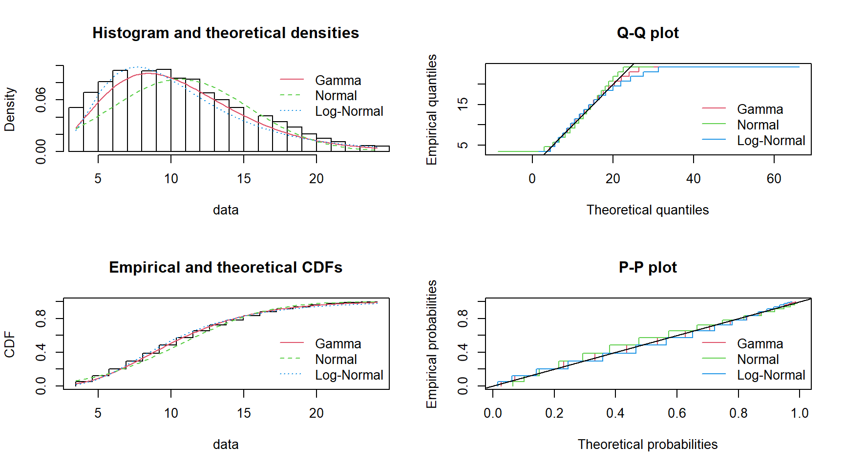
# Extract AIC and BIC values
results = tibble(
  Distribution = names(fits),
  AIC = sapply(fits, function(fit) fit$aic),
  BIC = sapply(fits, function(fit) fit$bic)
)

# Print the results table
print(results)
# A tibble: 3 × 3
Distribution AIC BIC
<chr> <dbl> <dbl>
1 Gamma 127152. 127168.
2 Normal 129622. 129638.
3 LogNormal 127740. 127756.Pressure
The density and CDF plots for the pressure show that the Normal distribution does a good job fitting the distribution of the data. The P-P plot indicates excellent agreement between the empirical and theoretical probabilities, suggesting the fit in the centre of the data is very good. The Q-Q plot shows some deviation at the far left and right of the plot, indicating the Normal distribution isn’t fitting well at the extreme values of the distribution tails. This is expected since the kurtosis of the data is slightly less than that of a Normal distribution.