Dataset: Red Portuguese “Vinho Verde” wine (Cortez et al., 2009)
The Data
Dataset: Red Portuguese “Vinho Verde” wine (Cortez et al., 2009)
Five input variables: citric acid, chlorides, total sulfur dioxide, pH, alcohol
One output variable: quality
Data Exploration
This section uses scatter plots to explore the relationship between wine quality and the independent variables citric acid, chlorides, total sulfur dioxide, and alcohol. Histogram plots of the dependent and independent variables are used to explore the distribution of each variable.
#(i) and (ii)data.raw=as.matrix(read.table("RedWine.txt"))set.seed(225259172)# the seed is my student ID number#(iii)subset.num_samples=460data.subset=data.raw[sample(1:1599, subset.num_samples), c(1:6)]data.variable.names=c("citric acid", "chlorides", "total sulfur dioxide", "pH", "alcohol")y.name='quality'#(iv)# Create 5 scatterplots function (for each X variable against the variable of interest Y)"colours=c("#9E9E9E","#61D04F","#2297E6","#CD0BBC","#F5C710","#DF536B")for(iinc(1,2,3,4,5)){name=data.variable.names[i]plot(x =data.subset[,i], y =data.subset[,6], col =colours[i], pch=20, cex=3, xlab=name, ylab=y.name, main=sprintf("Scatter plot of %s versus %s (n=%s)", y.name, name, subset.num_samples))}
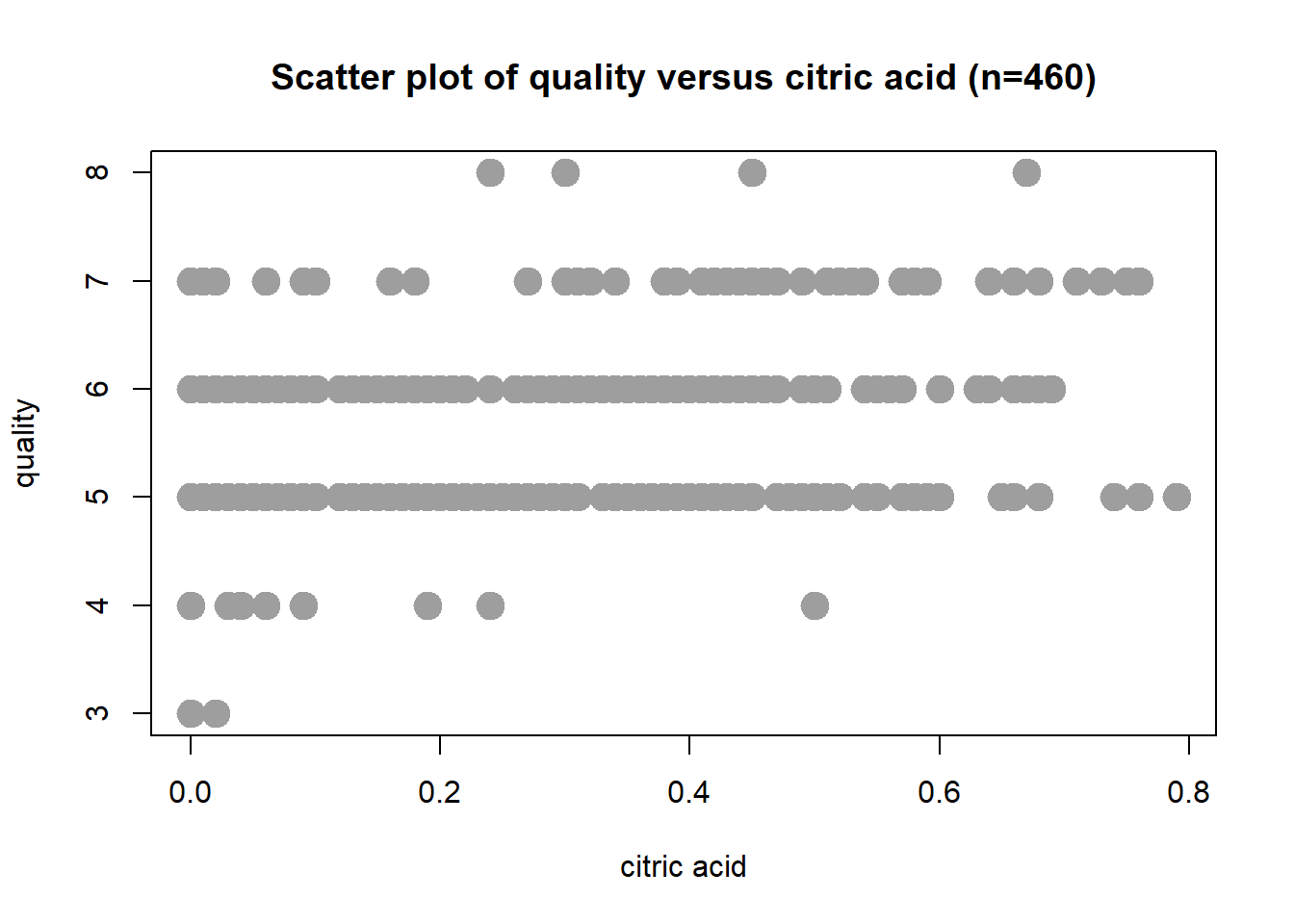
Scatter Plot: Citric Acid
Wine quality increases with increasing citric acid value. The correlation coefficient is r = 0.244.
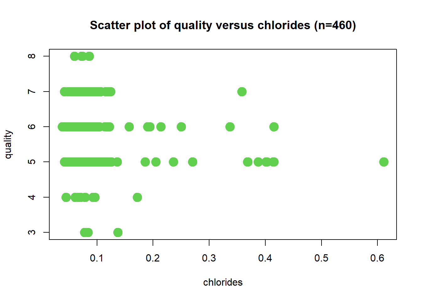
Scatter Plot: Chlorides
Wine quality decreases with increasing chlorides value. The correlation coefficient is r = -0.122. A potential outlier is observed at 0.61 chlorides value. A negation function will be required.
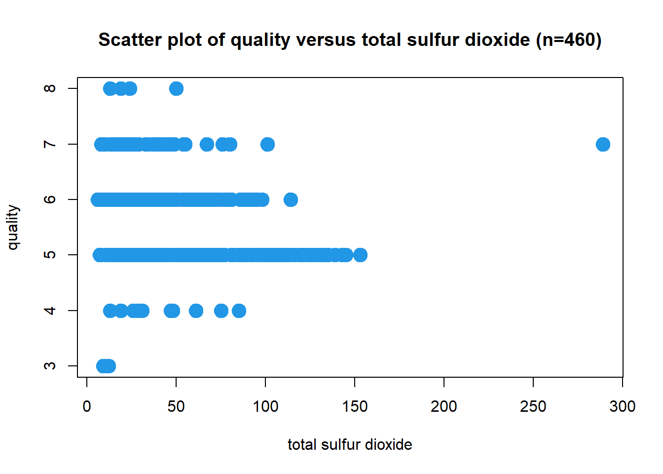
Scatter Plot: Total Sulfur Dioxide
Wine quality decreases with the increasing value of total sulphur dioxide. The correlation coefficient is r = -0.206. A possible outlier at a value of 289 for total sulfur dioxide. A negation function will be required.
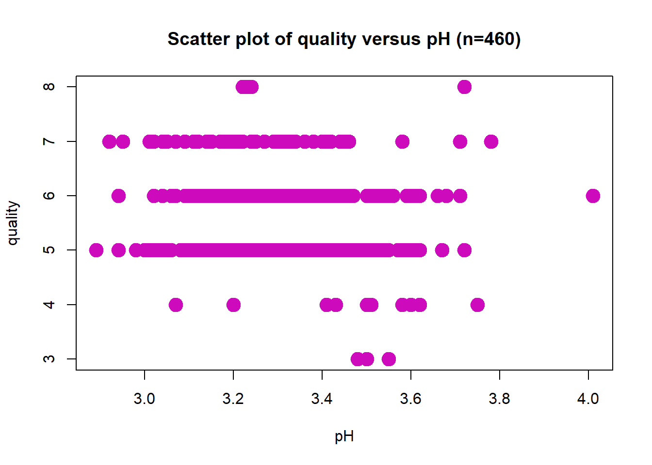
Scatter Plot: pH
Wine quality does not appear to have a linear relationship with pH. The correlation coefficient is r = -0.072. Potential outlier at pH value of 4.0.
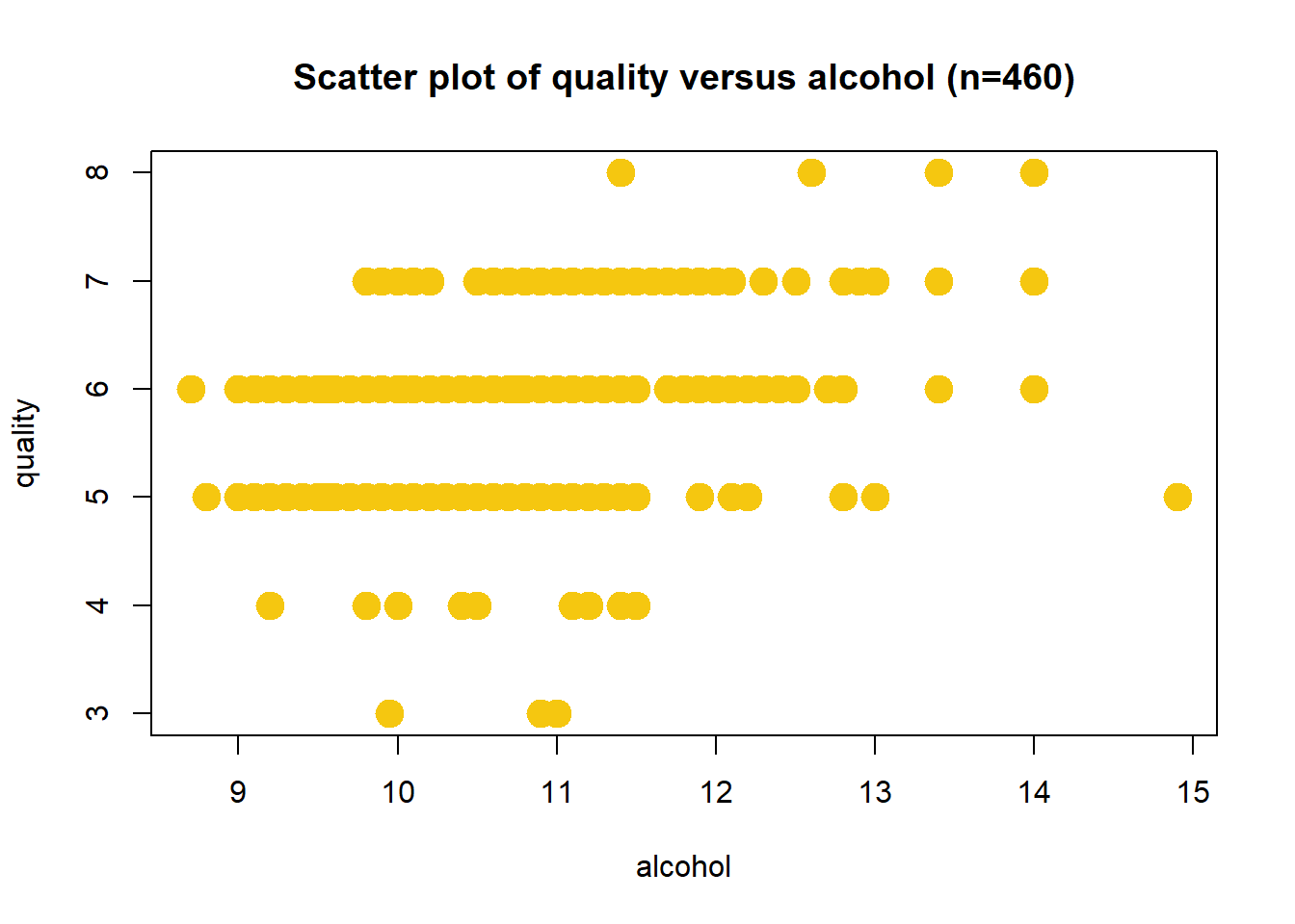
Scatter Plot: Alcohol
Wine quality increases with alcohol content. The correlation coefficient is r = 0.442.
# Number of bins for histogramsbins=c(16,30,48,11,24,8)# Create 6 histograms for each X variable and Yfor(iinc(1,2,3,4,5,6)){if(i==6){name=y.name}else{name=data.variable.names[i]}hist(data.subset[,i], breaks=bins[i], xlab=name, main=sprintf("Histogram of %s (n=%s)", name, subset.num_samples), col=colours[i])}
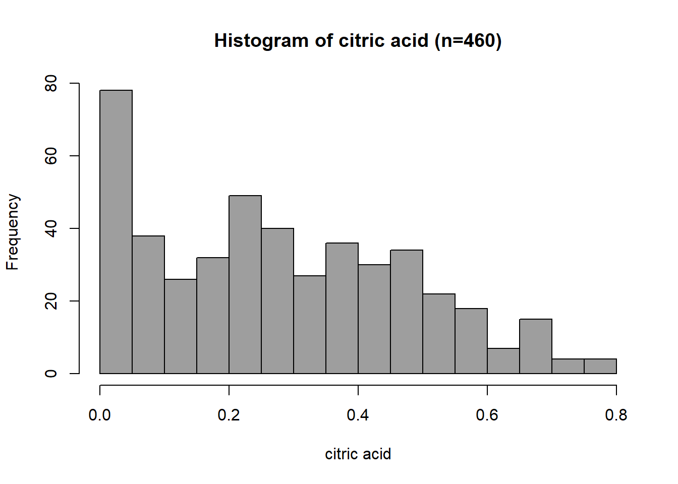
Histogram: Citric Acid
The distribution of citric acid is uniform for the middle values. However, many observations show a peak near-zero value. At the higher citric acid values, fewer observations give the distribution a right (positive) skew. The distribution range is from 0.000 to 0.790, with a median value of 0.260 and a mean of 0.284.
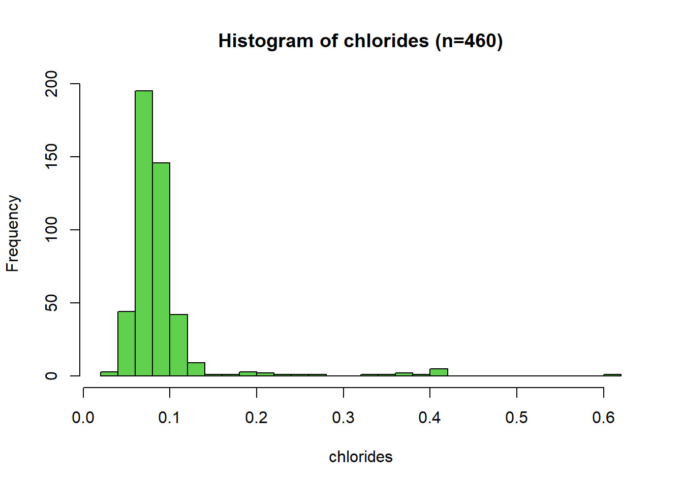
Histogram: Chlorides
The distribution of chlorides is unimodal with significant right (positive) skew. Most of the chlorides observations are between 0.04 and 0.15. Values above 0.15 have very few counts and are potential outliers. The distribution range is from 0.038 to 0.611, with a median value of 0.080 and a mean of 0.0912.
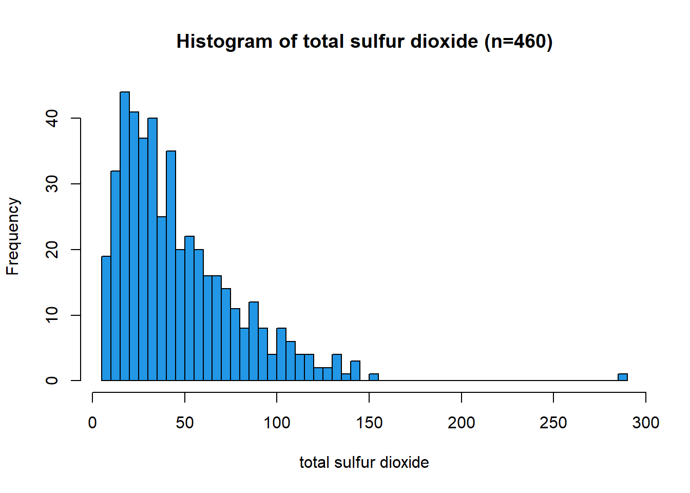
Histogram: Total Sulfur Dioxide
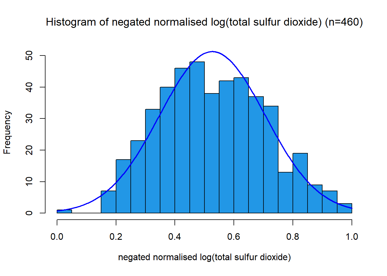
The distribution of total sulfur dioxide is unimodal with right (positive) skew and reassembles a log-normal shape. The value of 289 appears to be an outlier. The distribution range is from 6.0 to 289.0, with a median value of 38.5 and a mean of 47.12.
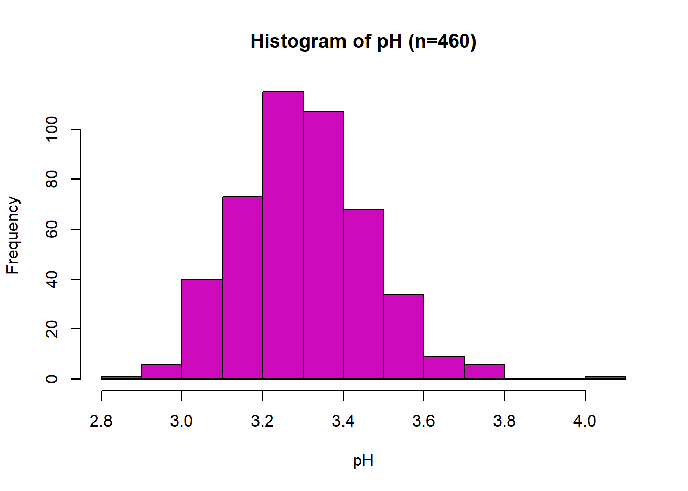
Histogram: pH
The distribution of pH is unimodal with minimal skew and a potential outlier at 4.01 and has a normal distribution shape. The distribution range is from 2.89 to 4.01, with a median value of 3.30 and a mean of 3.31.
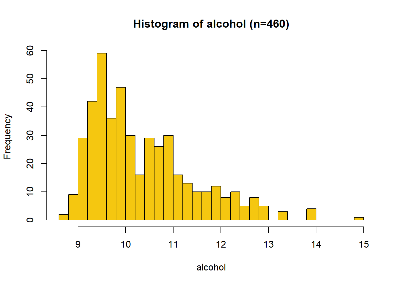
Histogram: Alcohol
The distribution of alcohol is unimodal with right (positive) skew and reassembles a log-normal shape. It ranges from 8.7 to 14.9, with a median value of 10.1 and a mean of 10.4.
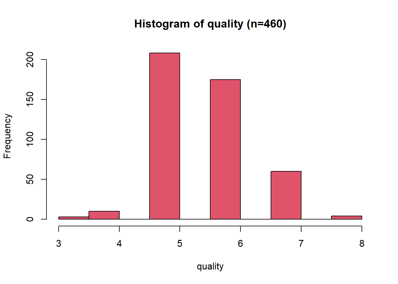
Histogram: Quality
The quality distribution is unimodal, with some right (positive) skew having a normal distribution shape. The data contains only integer values, which leads to gaps in the histogram unless a small number of bins are used. The distribution range is from 3 to 8, with a median value of 6 and a mean of 5.6.
# Generate a summary of the datasummary(data.subset)
       V1               V2                V3               V4
 Min.   :0.0000   Min.   :0.03800   Min.   :  6.00   Min.   :2.890
 1st Qu.:0.1000   1st Qu.:0.07100   1st Qu.: 23.00   1st Qu.:3.200
 Median :0.2600   Median :0.08000   Median : 38.50   Median :3.300
 Mean   :0.2837   Mean   :0.09117   Mean   : 47.12   Mean   :3.308
 3rd Qu.:0.4400   3rd Qu.:0.09400   3rd Qu.: 64.25   3rd Qu.:3.410
 Max.   :0.7900   Max.   :0.61100   Max.   :289.00   Max.   :4.010
       V5              V6
 Min.   : 8.70   Min.   :3.000
 1st Qu.: 9.50   1st Qu.:5.000
 Median :10.10   Median :6.000
 Mean   :10.41   Mean   :5.633
 3rd Qu.:11.00   3rd Qu.:6.000
 Max.   :14.90   Max.   :8.000
The independent variables citric acid, chlorides, total sulfur dioxide, and alcohol were chosen for the aggregation function fitting. These variables had the strongest association with wine quality. Treatment of outliers was considered, and it was decided not to apply any treatment.
library(e1071)# Required for Skewness functionlibrary(rcompanion)# Provides plotting of normal PDF on histogramlibrary(latex2exp)# Provides the ability to use latex in plot titles/labels # min-max normalisation# Allows optional arguements to set the min and max for the scalingminmax=function(x, x_min=NULL, x_max=NULL){if(is.null(x_min)){x_min=min(x)}if(is.null(x_max)){x_max=max(x)}(x-x_min)/(x_max-x_min)}# z-score standardisation and scaling to unit intervalunit.z=function(x){0.15*((x-mean(x))/sd(x))+0.5}# Negation function for normalised datanegation=function(x){(max(x)+min(x))-x}# Vector with indices of chosen variablesI=c(1,2,3,5,6)# Matrix containing the variables to transformvariables_for_transform=data.subset[,I]data.transformed=variables_for_transform
Citric acid
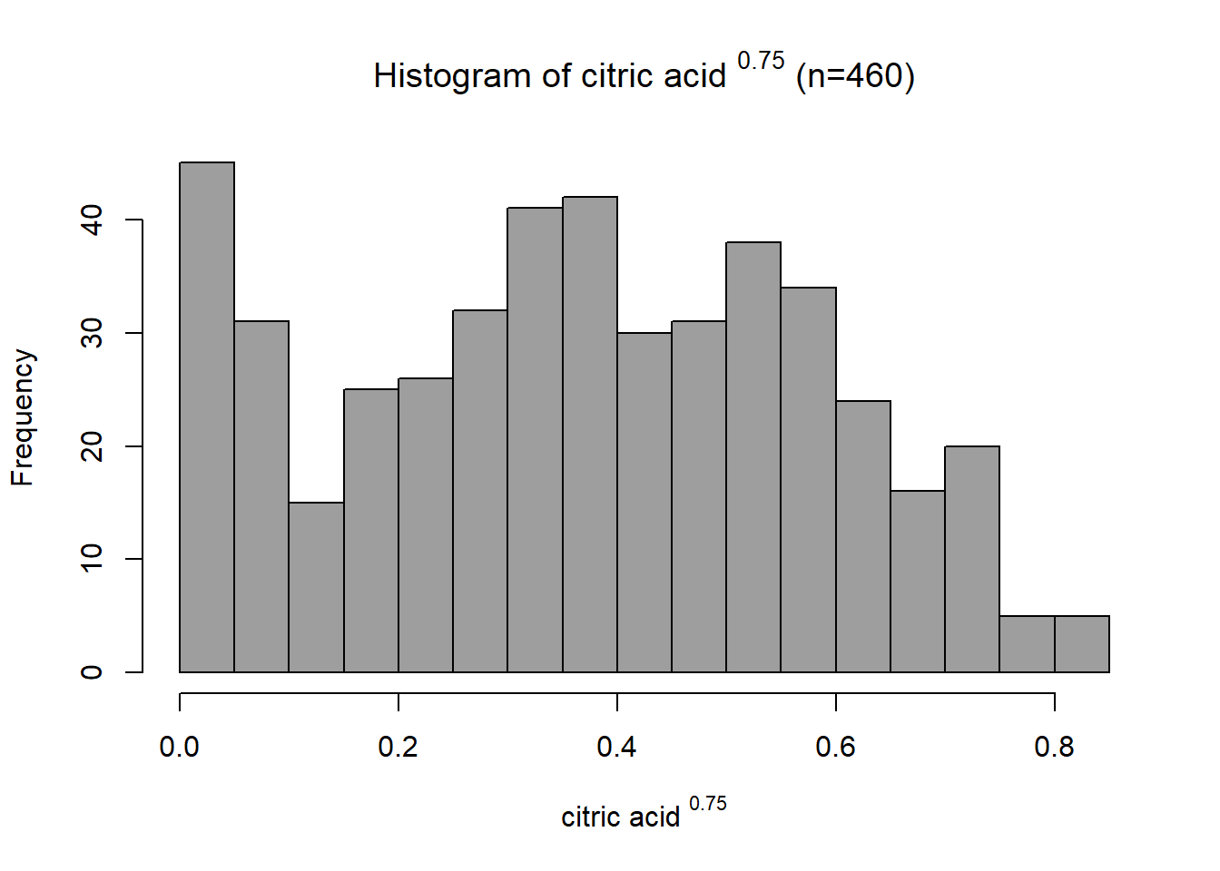
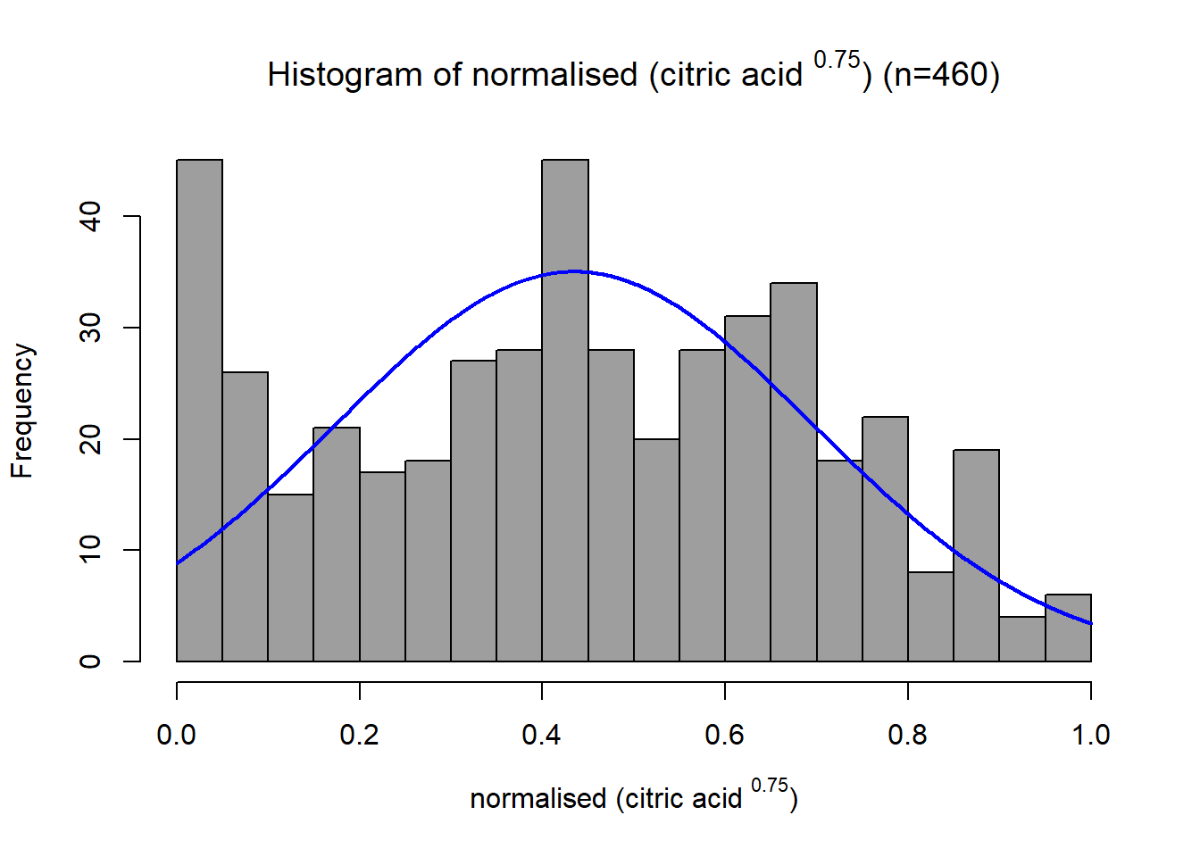
This distribution has some right skew with a skewness value of 0.326. Since the data is right-skewed, a power or log transformation is suitable. Through trial and error, the final transformation applied was \[x_{new} = x^{0.75}\]
This transformed the distribution closer to a normal distribution with a skewness of -0.04. The variable was then scaled between 0 and 1 using a min-max function. This variable already had a positive association with quality, so no negation was required.
# Transformp=0.75# final value after trying p=0.5 firstdata.transformed[,1]=variables_for_transform[,1]^pskewness(data.transformed[,1])
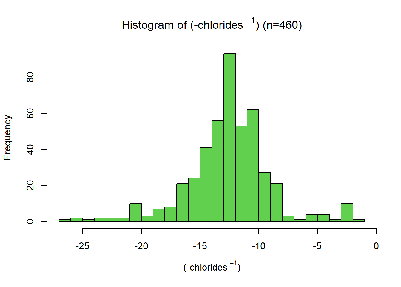
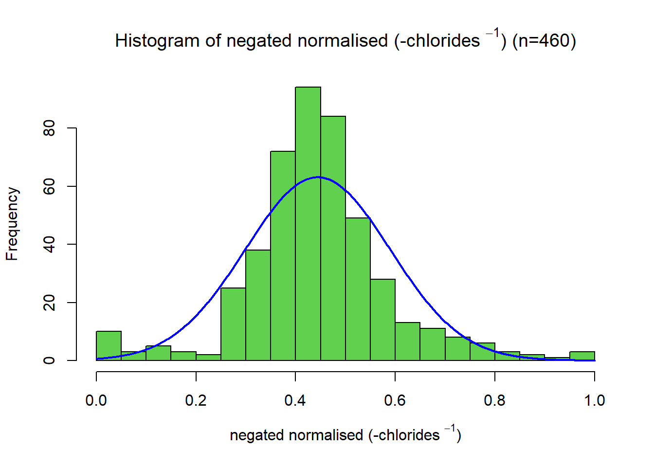
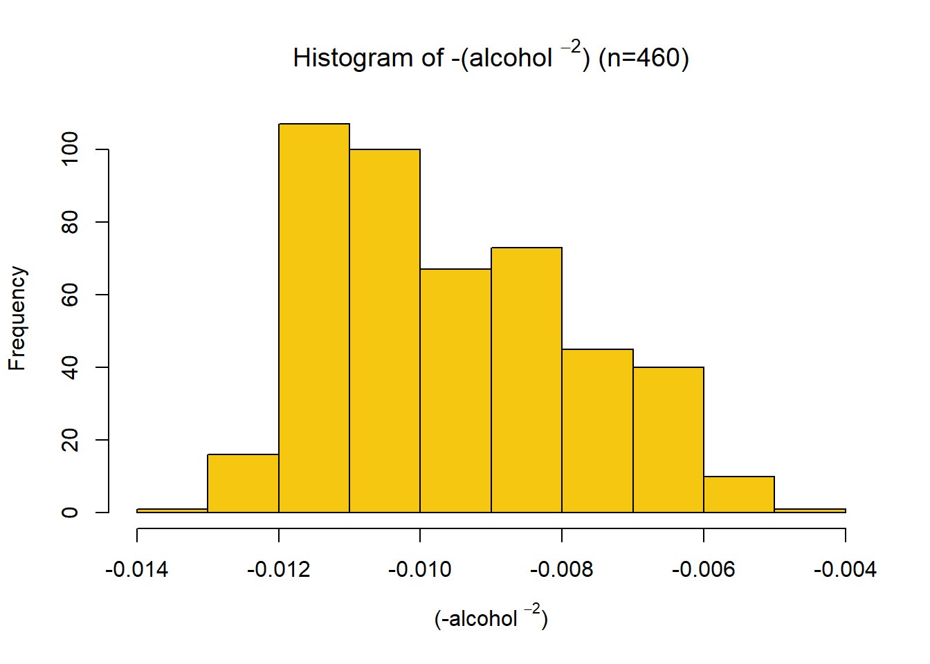
This distribution has a significant right skew, with a skewness value of 5.0. Since the data is right-skewed, a suitable transformation is a power or log transformation. A more substantial transformation than the log was required. Through trial and error, the final transformation applied was \[ x_{new} = -\frac{1}{x}\] Giving a skewness of -0.259.The variable was then scaled between 0 and 1 using a min-max function. This variable had a negative association with quality, so a negation function was applied.
# Transformp=-1# final value after trying log transform firstdata.transformed[,2]=-variables_for_transform[,2]^pskewness(data.transformed[,2])
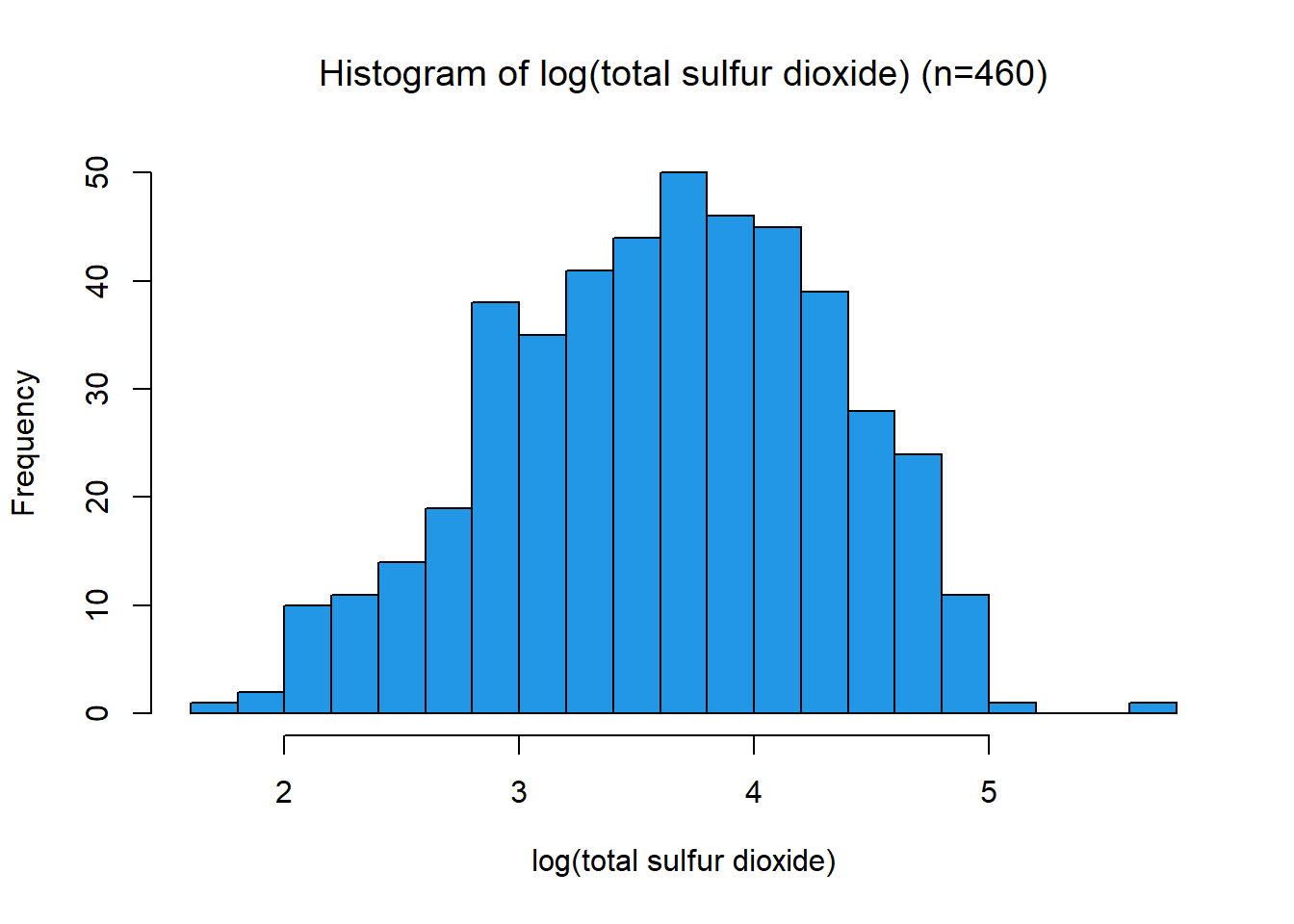
This distribution has a strong right skew, with a skewness value 1.72. Since the data is right-skewed, a suitable transformation is a power or log transformation. The distribution looks log-normal, the transformation applied was \[x_{new} = \log(x)\] This pushed the distribution closer to normal and reduced the skewness to -0.17. The variable was then scaled between 0 and 1 using a min-max function. This variable had a negative association with quality, so a negation function was applied.
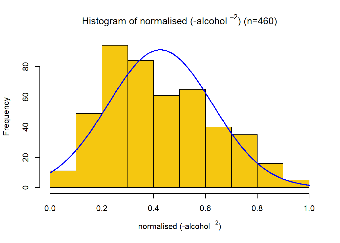
This distribution has a strong right skew, with a skewness value of 1.06. Since the data is right-skewed, a suitable transformation is a power or log transformation. The distribution looks log-normal, so a log transform was first tried. Through trial and error, the final transformation applied was \[x_{new} = -\frac{1}{x^2} \] Giving a skewness of -0.44. The variable was then scaled between 0 and 1 using a min-max function. This variable had a positive association with quality, so no negation was required.
# Transformp=-2# final valuedata.transformed[,4]=-(variables_for_transform[,4]^p)skewness(data.transformed[,4])
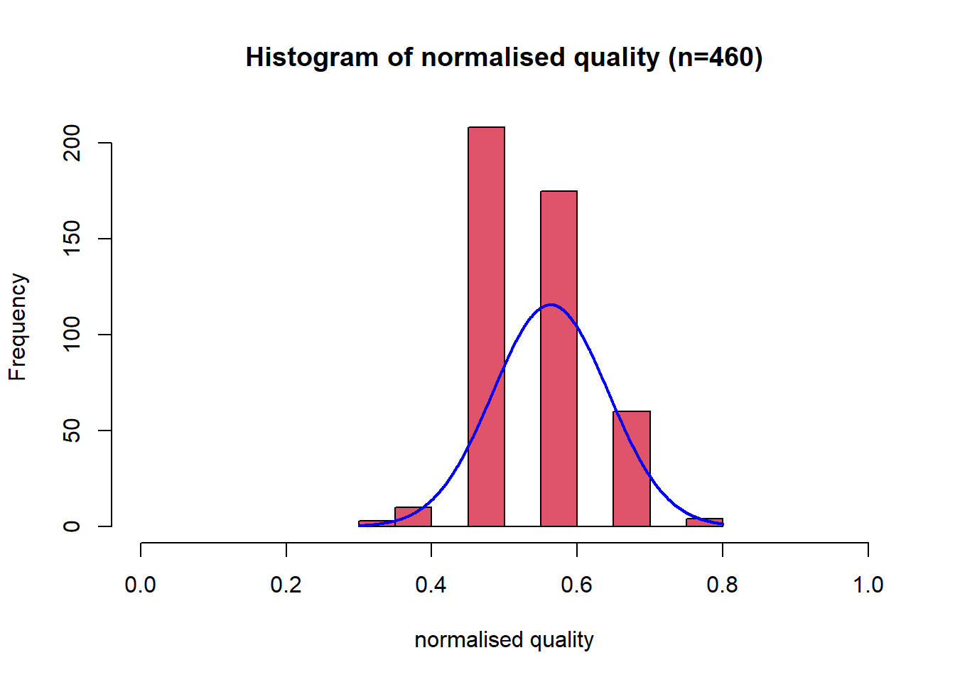
This distribution has some right skew, with a low skewness value of 0.28. Since the distribution already looks normal no data transformation was applied. The variable was then scaled between 0 and 1 using a min-max function. Using the range of possible values 0-10. This variable is the dependent variable, so no negation was required.
# Transform - no transformation applied to this variabledata.transformed[,5]=variables_for_transform[,5]skewness(data.transformed[,5])
[1] 0.2796584
name5=sprintf("%s", y.name)title5=sprintf("(Histogram of %s (n=%s))", y.name, subset.num_samples)hist(data.transformed[,5],xlab=name5, breaks=8, main=title5, col=colours[I[5]])
# We know the quality could range between 0 and 10, so use those values here.min_y=0max_y=10# Normalise between 0 - 1data.transformed[,5]=minmax(data.transformed[,5], min_y, max_y)name5s=sprintf("normalised %s", y.name)title5s=sprintf("Histogram of normalised %s (n=%s)", y.name, subset.num_samples)plotNormalHistogram(data.transformed[,5], xlab=name5s, breaks=8, main=title5s, col=colours[I[5]],xlim=c(0,1))
# Save this transformed data to a text filewrite.table(data.transformed, "stephens-transformed.txt")
Build models and investigate
A Weighted Arithmetic Mean (WAM), Weighted Power Mean (WPM) and Ordered Weighted Average (OWA) aggregation functions are fitted to the data for analysis and prediction using the AggWAfit R library of James (2016)
source("AggWaFit718.R")# Replace previous matrix with the one loaded from diskdata.transformed=as.matrix(read.table("stephens-transformed.txt"))# import saved data# Get weights for Weighted Arithmetic Mean with fit.QAM() fit.QAM(data.transformed,output.1="output_QAM_AM.txt",stats.1="stats_QAM_AM.txt",g=AM,g.inv=invAM)# Get weights for Power Mean p=0.5 with fit.QAM()fit.QAM(data.transformed,output.1="output_QAM_PM05.txt",stats.1="stats_QAM_PM05.txt",g=PM05,g.inv=invPM05)# Get weights for Power Mean p=2 with fit.QAM()fit.QAM(data.transformed,output.1="output_QAM_QM.txt",stats.1="stats_QAM_QM.txt",g=QM,g.inv=invQM)# Get weights for Ordered Weighted Average with fit.OWA()# Note that in AddWaFit the weights don't correspond to the variables but their relative sizes.fit.OWA(data.transformed,output.1="output_OWA.txt",stats.1="stats_OWA.txt")
Model Results
Metric
WAM
WPM (0.5)
WPM (2)
OWA
RMSE
0.1403
0.1525
0.1279
0.1204
Avg Abs Error
0.1187
0.1258
0.1070
0.0985
Pearson
0.3373
0.2823
0.3857
0.4130
Spearman
0.3602
0.3179
0.3973
0.4217
Model Weights
Weight
WAM
WPM (0.5)
WPM (2)
OWA (orness=0.72)
w1
0.1589
0.0290
0.2346
0.0590
w2
0.3413
0.3772
0.3241
0.2098
w3
0.4750
0.5632
0.3233
0.2537
w4
0.0247
0.0306
0.1179
0.4775
Model Insights
Importance of each variable
From the WAM and WPM models
The chlorides (32-37%) and total sulfur content (32-56%) are the most important variables. A majority of the models weight citric acid (3-23%) as more important than alcohol (2.5 to 11%).
OWA weights correspond with each input’s relative size, not the input’s source. The orness value of 0.72 suggests more weight is allocated to the higher inputs. The last weight indicates approximately 48% of the weight is allocated to the largest input.
The OWA model best fits the selected data, giving the lowest RMSE and highest correlation coefficients. On average, the prediction is out by ~ 10%
Use Model for Prediction
new_input<-c(0.8, 0.63, 37, 2.51, 7.0)new_input_for_transform<-new_input[c(1,2,3,5)]# choose the same four X variables as in Q2 # Note: some of these values are outside the min/max that were used when transforming the data before fitting.# It was recommended to just use a new min/max for these variables here incorporating the values from new_input.# Transforming the four variables in the same way as in question 2new_input_transformed=new_input_for_transform############## citric acid############## Transformnew_input_transformed[1]=new_input_for_transform[1]^0.75# Normalise between 0 - 1new_input_transformed[1]=minmax(new_input_transformed[1], min(c(min_1,new_input_transformed[1])), max(c(max_1,new_input_transformed[1])))############ chlorides############ Transformnew_input_transformed[2]=-new_input_for_transform[2]^-1# Normalise between 0 - 1new_input_transformed[2]=minmax(new_input_transformed[2], min(c(min_2,new_input_transformed[2])), max(c(max_2,new_input_transformed[2])))# Negatenew_input_transformed[2]=negation(new_input_transformed[2])####################### total sulfur dioxide####################### Transformnew_input_transformed[3]=log(new_input_for_transform[3])# Normalize between 0 - 1new_input_transformed[3]=minmax(new_input_transformed[3], min(c(min_3,new_input_transformed[3])), max(c(max_3,new_input_transformed[3])))# Negatenew_input_transformed[3]=negation(new_input_transformed[3])####################### alcohol####################### Transformnew_input_transformed[4]=-new_input_for_transform[4]^-2# Normalize between 0 - 1new_input_transformed[4]=minmax(new_input_transformed[4], min(c(min_4,new_input_transformed[4])), max(c(max_4,new_input_transformed[4])))# Applying the transformed variables to the best model selected from Q3 for Y prediction# Weights from best fitting model (OWA)Xweights=c(0.0590,0.2098,0.2537,0.4775)y_pred=OWA(new_input_transformed, Xweights)# Reverse the transformation to convert back the predicted Y to the original scale and then round it to integer####################### quality####################### Normalise between 0 - 1predicated_quality=round(y_pred*(max_y-min_y)+min_y)
Prediction Example
Variable
Raw
Transformed
Citric Acid
0.8
1
Chlorides
0.63
1
Total Sulfur Dioxide
37
0.47
Alcohol
7.0
0
Predicted Quality: 8 (too high) - The quality prediction is too high and, therefore, unreasonable - High orness means only a few high inputs would give a high output (quality)
Best conditions for higher-quality wine
Higher values for the inputs: citric acid, negation(chlorides), negation (total sulfur dioxide), alcohol
Higher – citric acid and alcohol
Lower – chlorides and total sulfur dioxide
Limitations, Ethics & Privacy
Limitations of the fitting model
Correlation coefficients are weak
OWA doesn’t tell you the importance of the variables
The model is only as good as the training data
The predicated value was beyond the training data set for 3 of the 4 variables
The data does not raise privacy concerns as it does not contain information about grape types, wine brands, wine prices, etc. Only de-identified data is used.
Professional ethics
Transparent about the methods used to analyse the data
R script provided that documents all assumptions and steps
Raw and transformed data is available
References
Cortez P, Cerdeira A, Almeida F, Matos T and Reis J (2009) ‘Modeling wine preferences by data mining from physicochemical properties’. Decision Support Systems, 47(4):547-553.
Csárdi G, Berkelaar M (2024) lpSolve: Interface to ‘Lp_solve’ v. 5.5 to Solve Linear/Integer Programs [R package], v5.6.23, accessed 3 April 2025. https://github.com/gaborcsardi/lpSolve
Mangiafico S S (2025) rcompanion: Functions to Support Extension Education Program Evaluation [R package], v2.5.0, Rutgers Cooperative Extension, accessed 3 April 2025. https://CRAN.R-project.org/package=rcompanion/
Meschiari S (2024). latex2exp: Use LaTeX Expressions in Plots [R package], v0.9.8, accessed 3 April 2025. https://www.stefanom.io/latex2exp/.
Meyer D, Dimitriadou E, Hornik K, Weingessel A and Leisch F (2024) e1071: Misc Functions of the Department of Statistics, Probability Theory Group (Formerly: E1071), TU Wien [R package]. v1.7-16, accessed 3 April 2025. https://CRAN.R-project.org/package=e1071.
James, S (2016). AggWAfit R library. 10.13140/RG.2.1.1906.9688.