Real Estate Price Prediction

import os
import json
import numpy as np
import matplotlib.pyplot as plt
import matplotlib.ticker as ticker
import pymupdf
import pandas as pd
import re
import time
import seaborn as sns
from geopy.geocoders import Nominatim
from geopy.distance import geodesic
from geopy import Point
from sklearn.model_selection import train_test_split, GridSearchCV
from sklearn.preprocessing import OneHotEncoder, StandardScaler
from sklearn.compose import ColumnTransformer
from sklearn.pipeline import Pipeline
from sklearn.linear_model import ElasticNet
from sklearn.model_selection import cross_validate, learning_curve
from sklearn.model_selection import cross_val_score
from sklearn.metrics import r2_score, root_mean_squared_error, mean_absolute_error
from sklearn.neighbors import KNeighborsRegressor
from sklearn.ensemble import RandomForestRegressor
from sklearn.inspection import permutation_importance
import shap

#import warnings

# Set the style for seaborn
sns.set_theme(style="whitegrid")

Introduction

The task required the selection of three suburbs on which to collect housing data. The chosen suburbs were:

• Berwick
• Officer
• Pakenham # Melbourne Housing Data acquisition Data collection leveraged realestate.com.au using the process described below. The goal was to obtain at least 150 data points (50 for each suburb). As the number of data points is low, it was decided to focus on the period between January to August 2025. Two property types were considered for his task, houses and townhouses. These suburbs on the outer edge of metropolitan Melbourne and other property types such as units and apartments are not as popular and have very low sales volumes.

Data Ethics and privacy

The data is this task is publicly available on a number of property websites and contains no personal identifying information about the sellers or buyers. The source of the data, on the other hand did raise some ethical issues. Data was sourced from the realestate.com.auau/) website as required in the task specifications. The terms and conditions for usage of the realestate.com.au website prohibits the use of “any automated device, software, process or means to access, retrieve, scrape, or index our Platforms or any content on our websites.”. Therefore, any automated approach that directly scraped data from the website would be in violation of the terms and conditions of the websites use. The approach adopted in this work involved manually perusing the website and printing the result to a PDF file. The contents of the PDF file could then be extracted automatically.

Data collection process

The steps involved in the data collection process were:

1. For each of the chosen suburbs, search for sold properties. Limiting the search to only those properties with a sold price, and type of property i.e. house or townhouse and sold in the last 12 months.

2. For each page of the search results within the required Jan to Aug period, print to a PDF file.

3. Combine all PDF documents for each suburb and property type into a single PDF file.

4. Process the PDF using the created Python code. The steps of the python code are:

   1. Read the PDF file using the pymupdf package.

   2. For every page in the document extract the text and join the text together in a large single string.

   3. Use a regular expression patterns to split the full text into a list of blocks. The regular expression pattern looked for new line character followed by a dollar sign ($). This signifies the start of a listing block.

   4. Define regular expression patterns to identify the price, address, property details such as number of bedrooms, bathrooms, car spaces and land size, sold date, and property type.

   5. For each listing block of text find all text that matches the patterns in (step d).

   6. For all the found patterns, process them and store them into a dictionary for this listing. Appending the dictionary to a list of listings.

   7. After all of the listing blocks have been processed, convert the listings list into a DataFrame.

   8. Check for and handle missing data. Some real estate listing do not include the land size. Rather than skipping these, it was decided to included them and then impute the missing land size from the median. Since townhouses have a much lower median land size than houses, the imputation of missing land size was done per property type.

   9. Store the DataFrame for the suburb.

# Functions for extracting real estate data from PDF's
def split_address(address):
    """
    Function that takes an address string and splits it into its components. Handling two
    or three components.

    :param address:
    :returns: Tuple with the street address and the suburb.
    """
    parts = address.split(", ")
    if len(parts) >= 2:
        street = ", ".join(parts[:-1])  # everything except the last part
        sub = parts[-1]              # last part
        return street, sub
    else:
        return address, "unknown"       # fallback if format is unexpected


def process_pdf(pdf_file):
    """
    Function to extract real estate data from a PDF. The function assumes the PDF has been
    printed from the realestate.com.au website.

    :param pdf_file: File name and path to pdf.
    :returns: DataFrame with extracted data.
    """
    # Open the PDF file
    doc = pymupdf.open(pdf_file)

    # Combine all text from the PDF
    # Makes sure listing that are split across pages are captured
    full_text = ""
    for page in doc:
        full_text += page.get_text() + "\n"

    # Split the full text into chunks that likely represent individual listings
    # Looks for a newline followed by a price pattern
    listing_blocks = re.split(r"\n(?=\$\d[\d,]*)", full_text)

    # Regular expression patterns to extract relevant data
    # Matches dollar amounts that start with a dollar sign, have at least one digit, and
    # can contain additional digits and commas in any combination.
    price_pattern = re.compile(r"\$(\d[\d,]*)")

    # Text that starts with one or more digits, followed by any characters, and ends with
    # one of the three specified words.
    address_pattern = re.compile(r"\d+.*, (?:Officer|Berwick|Pakenham)",
                                 re.IGNORECASE)

    # Match strings containing four pieces of information separated by whitespace,
    # bedrooms, bathrooms, garages and area measurement in square meters or hectares.
    # Match even if the area is missing

    details_pattern = re.compile(
        r"(\d+)\s+(\d+)\s+(\d+)(?:\s+([\d,]+(?:\.\d+)?)(m²|ha))?"
    )

    # Look for date formats following "Sold on", specifically in the format of day-month-year
    # where the month is abbreviated with 3 characters.
    sold_date_pattern = re.compile(r"Sold on (\d{2} \w{3} \d{4})")

    # Match any of these four exact words representing the types of properties.
    property_type_pattern = re.compile(r"House|Townhouse")

    # List to store extracted data
    listings = []

    # Iterate through each page in the PDF
    for block in listing_blocks:
        # Extract prices using regex
        prices = price_pattern.findall(block)

        # Extract address using regex
        addresses = address_pattern.findall(block)

        # Extract the property details, bedrooms, bathrooms, cars and area
        details = details_pattern.findall(block)

        # Extract sold date
        sold_dates = sold_date_pattern.findall(block)

        # Extract the property type
        property_types = property_type_pattern.findall(block)

        # Loop through the listing found on this page to store the information
        # prices, address or details might be empty for a listing if not all the
        # information is found. This is common for details where the land area is missing.
        # Only lists where the complete information is found are added to the dataframe.

        if sold_dates and property_types and prices and addresses and details:

            bedrooms, bathrooms, car_spaces, land_size, land_size_unit = details[0]

            # Split the address into street and suburb
            street_address, sub = split_address(addresses[0])

            # Handle comma in number
            land_size = float(land_size.replace(",", "")) if land_size else np.nan

            if land_size_unit == 'ha':
                land_size = land_size*10000

            listing = {
                "sold_price": int(prices[0].replace(",", "")) ,
                "address": street_address,
                "suburb" : sub,
                "bedrooms": int(bedrooms),
                "bathrooms": int(bathrooms),
                "car_spaces": int(car_spaces),
                "land_size": land_size,
                "property_type": property_types[0],
                "sold_date": sold_dates[0]
            }
            listings.append(listing)

    return pd.DataFrame(listings)

def select_samples(df, num_samples):
    """
    Randomly select the required number of samples stratified on the property type.

    :param df: Dataframe with data to sample.
    :param num_samples: The number of samples to select.
    :return: Dataframe with selected samples.
    """
    # Stratify and randomly select
    sample_df, _ = train_test_split(
        df, train_size=num_samples, stratify=df["property_type"], random_state=0
    )

    return sample_df

A total of three DataFrames were obtained after executing the above process, one for each suburb. Since the data was extracted to cover the period January to August 2025, each DataFrame contained more than the required number of data points.

suburbs = ["Berwick", "Officer", "Pakenham"]

# Set sampling to uniform
sampling_option = "uniform"

suburb_data = {}
suburb_totals = {}

for suburb in suburbs:
    print(f"\nProcessing suburb: {suburb}")

    suburb_name = suburb.lower()

    # Process pdf
    suburb_df = process_pdf(f"data/{suburb_name}.pdf")

    # Ensure dateTime object
    suburb_df["sold_date"] = pd.to_datetime(suburb_df["sold_date"])

    # Detect and analyse missing values
    missing_count = suburb_df.isnull().sum().astype(int)
    missing_percentage = round(suburb_df.isnull().mean() * 100, 2)

    # Create a DataFrame
    missing_df = pd.DataFrame(
        {"missing_count": missing_count, "missing_percentage": missing_percentage}
    )

    # Check the number of missing values for the numerical features
    print("Missing value count per feature:")
    print(missing_df)

    # Group by property type and count missing values for each column
    missing_values_by_type = suburb_df.groupby("property_type")["land_size"].apply(
        lambda x: x.isna().sum()
    )

    # Display the result
    print("\nNumber of missing land size's per property type:")
    for ix, val in missing_values_by_type.items():
        print(f"{ix} {val}")

    # Calculate the median land_size for each property type
    median_land_size = suburb_df.groupby("property_type")["land_size"].median()
    print("\nMedian land size per property type:")
    for ix, val in median_land_size.items():
        print(f"{ix} {val}")

    # Impute missing land_size values with the median for each property type
    suburb_df["land_size"] = suburb_df.apply(
        lambda row: median_land_size[row["property_type"]] if pd.isna(row["land_size"]) else row["land_size"],
        axis=1
    )

    # Add the number of sales to the total dictionary
    suburb_totals[suburb] = suburb_df.shape[0]

    # Store the DataFrame
    suburb_data[suburb]= suburb_df

# Create a DataFrame for printing
suburb_totals_df = pd.DataFrame.from_dict(suburb_totals,
                                          orient="index", columns=["Total Sales"])
# Print suburb total
print()
print(suburb_totals_df.to_string(index=True))

if sampling_option == "proportional":
    # Find the suburb with the smallest total
    min_suburb = min(suburb_totals, key=suburb_totals.get)
    min_total = suburb_totals[min_suburb]

    # Set the sample size for the smallest suburb to 60
    base_sample_size = 60

    # Calculate the sample sizes for each suburb maintaining the relative ratios
    sample_sizes = {
        suburb: round((total / min_total) * base_sample_size)
        for suburb, total in suburb_totals.items()
    }

else:
    # Calculate the uniform sample sizes
    sample_sizes = {
        suburb: 60 for suburb, total in suburb_totals.items()
    }

suburb_totals_df["Number of Samples"] = suburb_totals_df.index.map(sample_sizes)

# Display the calculated sample sizes
print()
print(suburb_totals_df.to_string(index=True))

# Sample suburb data.
sampled_suburb_data = []
print("\nSampling suburb data.")
for suburb in suburbs:
    n_samples  = suburb_totals_df.loc[suburb, "Number of Samples"]
    print(f"Selecting {n_samples} points from {suburb}")
    sampled_suburb_data.append(select_samples(suburb_data[suburb], n_samples))

# Combine all DataFrames into one
red_df = pd.concat(sampled_suburb_data, ignore_index=True)

red_df.head()

Processing suburb: Berwick
Missing value count per feature:
               missing_count  missing_percentage
sold_price                 0                0.00
address                    0                0.00
suburb                     0                0.00
bedrooms                   0                0.00
bathrooms                  0                0.00
car_spaces                 0                0.00
land_size                108               21.39
property_type              0                0.00
sold_date                  0                0.00

Number of missing land size's per property type:
House 91
Townhouse 17

Median land size per property type:
House 612.0
Townhouse 195.1

Processing suburb: Officer
Missing value count per feature:
               missing_count  missing_percentage
sold_price                 0                0.00
address                    0                0.00
suburb                     0                0.00
bedrooms                   0                0.00
bathrooms                  0                0.00
car_spaces                 0                0.00
land_size                 81               23.82
property_type              0                0.00
sold_date                  0                0.00

Number of missing land size's per property type:
House 74
Townhouse 7

Median land size per property type:
House 400.0
Townhouse 164.8

Processing suburb: Pakenham
Missing value count per feature:
               missing_count  missing_percentage
sold_price                 0                0.00
address                    0                0.00
suburb                     0                0.00
bedrooms                   0                0.00
bathrooms                  0                0.00
car_spaces                 0                0.00
land_size                131               19.49
property_type              0                0.00
sold_date                  0                0.00

Number of missing land size's per property type:
House 110
Townhouse 21

Median land size per property type:
House 541.0
Townhouse 138.0

          Total Sales
Berwick           505
Officer           340
Pakenham          672

          Total Sales  Number of Samples
Berwick           505                 60
Officer           340                 60
Pakenham          672                 60

Sampling suburb data.
Selecting 60 points from Berwick
Selecting 60 points from Officer
Selecting 60 points from Pakenham

	sold_price	address	suburb	bedrooms	bathrooms	car_spaces	land_size	property_type	sold_date
0	630000	4 Lavender Place	Berwick	2	2	2	324.0	House	2025-03-03
1	970000	32 Bridgewater Boulevard	Berwick	4	2	2	606.0	House	2025-04-01
2	1000000	28 Bridgewater Boulevard	Berwick	5	2	2	608.0	House	2025-03-20
3	967500	1/4A Buchanan Road	Berwick	3	2	2	312.0	House	2025-06-28
4	1160000	9 Lowanna Street	Berwick	4	2	2	592.0	House	2025-08-19

## Plot Distribution of proportions across suburbs in the original and sampled data
# Calculate suburb proportions in the sampled data
sample_suburb_proportions = red_df["suburb"].value_counts(normalize=True)

# Calculate proportions in original data
total_original = sum(suburb_totals.values())
original_proportions = {k: v / total_original for k, v in suburb_totals.items()}

# Create a DataFrame for plotting
plot_df = pd.DataFrame({
    "Suburb": suburbs,
    "Sample": [sample_suburb_proportions.get(suburb, 0) for suburb in suburbs],
    "Original": [original_proportions.get(suburb, 0) for suburb in suburbs]
})

# Plot side-by-side bar chart
bar_x = range(len(suburbs))
width = 0.35

bar_fig, bar_ax = plt.subplots()
bar_ax.bar([i - width/2 for i in bar_x], plot_df["Sample"], width, label="Sample")
bar_ax.bar([i + width/2 for i in bar_x], plot_df["Original"], width, label="Original")

bar_ax.set_xticks(bar_x)
bar_ax.set_xticklabels(suburbs)
bar_ax.set_ylabel("Proportion")
bar_ax.set_title("Proportion of Sales Across Suburbs")
bar_ax.legend()

plt.tight_layout()
plt.savefig("images/suburb_proportion_comparison.png")
plt.show()

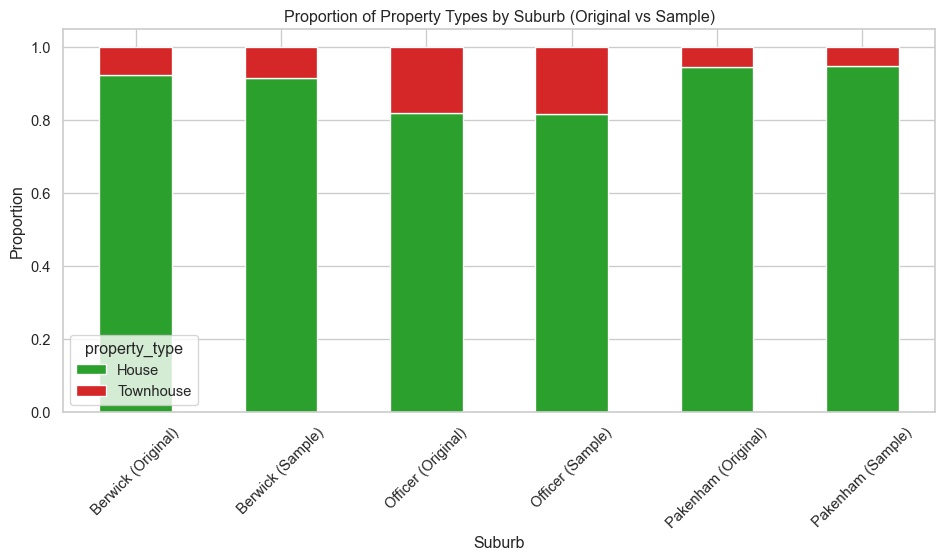
## Plot Distribution of property types in sample vs original data
# Function to calculate proportions
def calculate_proportions(df, sub_name, source_label):
    counts = df["property_type"].value_counts(normalize=True)
    result = counts.to_frame().reset_index()
    result.columns = ["property_type", "proportion"]
    result["suburb"] = f"{sub_name} ({source_label})"
    return result

# Process original data
original_results = []
for suburb, df_suburb in suburb_data.items():
    original_results.append(calculate_proportions(df_suburb, suburb, "Original"))

# Process sample data
sample_results = []
for suburb in red_df["suburb"].unique():
    subset = red_df[red_df["suburb"] == suburb]
    sample_results.append(calculate_proportions(subset, suburb, "Sample"))

# Combine all results
combined_df = pd.concat(sample_results + original_results, ignore_index=True)

# Pivot for stacked bar chart
pivot_df = combined_df.pivot(index="suburb", columns="property_type", values="proportion").fillna(0)

# Plotting
pivot_df.plot(kind="bar", stacked=True, figsize=(10, 6), color=["tab:green", "tab:red"])
plt.ylabel("Proportion")
plt.title("Proportion of Property Types by Suburb (Original vs Sample)")
plt.xticks(rotation=45)
plt.xlabel("Suburb")
plt.tight_layout()
plt.savefig("images/property_type_proportions_comparison.png")
plt.show()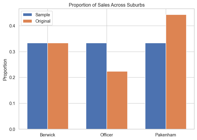

Data preprocessing and exploratory data analysis

Feature engineering

Additional features are added to the already collected data. The additional features considered in this work are:

• The number of primary and secondary schools within an X km radius,
• The number of child care services within an X km radius,
• The distance to the nearest training station,
• The distance to the nearest bus stop,
• The distance to the nearest shopping centre,
• The distance to the nearest park,
• The month of the year sold as cosine and sine,
• The day of the week sold,
• The number of days since January 1st 2025.

The first six features require the geographic location for each property and converts it into features that might be meaningful for buyers. The last three feature helps include the sold data information into the models by including a time based features. Prices today are most likely different from prices weeks or month ago. Each of these features requires additional data and processing steps. These are discuss in the following sections.

Obtaining latitude and longitude

The geopy package is used to obtain the latitude and longitude of a location. Geopy provides a client interface for several popular geocoding web services. The Nominatim web service was utilised as it is free. Nominatim uses OpenStreetMap data to find locations on Earth by name and address. The only limitations found were that it required only one request per second and could time out. A time-out value of 60 seconds was found to work.

Two functions were created, geocode_addresses() and geocode_address(), this first operates on DataFrames and calls the second function to convert the address into a latitude/longitude tuple. For efficiency, the data is saved into a CSV file so if the function is run multiple times it will only process the data once and read it from the saved data for subsequent calls.

# Functions to geocode address information into latitude and longitude
def geocode_address(address, state="Victoria"):
    """
    Function to return the latitude and longitude a given address.
    If no latitude or longitude can be found for the provided address,
    then None is returned.

    :param address: String containing the street address with suburb
    :param state: String containing the name of state for the address
    :return: Latitude and longitude tuple
    """
    geocoder = Nominatim(user_agent="geocoder")
    try:
        # Add ", Victoria, Australia" to improve geocoding accuracy
        full_address = f"{address}, {state}, Australia"
        location = geocoder.geocode(full_address)
        if location:
            return location.latitude, location.longitude
        else:
            return None, None
    except Exception as e:
        print(f"Geocoding error for {address}: {e}")
        return None, None

def geocode_addresses(data_df, file_name, address_key, suburb_key):
    """
    Function to process all addresses in a dataframe and return a dataframe containing the
    address and the latitude and longitude.

    :param data_df: Pandas DataFrame containing the addresses.
    :param file_name: String containing the file name.
    :param address_key: String containing the address key.
    :param suburb_key: String containing the suburb key.
    :return: Pandas DataFrame containing the address and the latitude and longitude.
    """
    geo_location_file = os.path.join("data", file_name)
    if os.path.exists(geo_location_file):
        print(f"File '{geo_location_file}' exists.")
        print(f"Reading geo locations.")
        addresses_geo = pd.read_csv(geo_location_file, comment="#")
    else:
        print(f"File '{geo_location_file}' does not exist.")
        print("Creating geo locations.")

        # Geocode each address with a delay to respect rate limits
        results = []

        for index, row in data_df.iterrows():
            # Create free form address
            addrs = row[address_key] + ", " + row[suburb_key]
            # Retrieve lat and long
            lat, lon = geocode_address(addrs)
            # Store results
            results.append({
                address_key: row[address_key],
                "latitude": lat,
                "longitude": lon
            })
            time.sleep(1)  # Respect Nominatim's rate limit

        # Create dataframe from results
        addresses_geo = pd.DataFrame(results)

        # Drop and location where a latitude or longitude was not found
        addresses_geo = addresses_geo.dropna(subset=["latitude", "longitude"])
        addresses_geo.to_csv(geo_location_file, index=False)

        print(f"Results saved to {geo_location_file}.")

    # Join the geo addresses to the loaded dataframe
    geodata_df = pd.merge(data_df, addresses_geo, how="inner", on=address_key)

    print("Geocoding complete.")
    return geodata_df

# geocode the addresses for the real estate date
red_geo_df = geocode_addresses(red_df, file_name="geocoded_addresses.csv",
                                  address_key="address", suburb_key="suburb")
red_geo_df.head(10)

File 'data\geocoded_addresses.csv' exists.
Reading geo locations.
Geocoding complete.

	sold_price	address	suburb	bedrooms	bathrooms	car_spaces	land_size	property_type	sold_date	latitude	longitude
0	630000	4 Lavender Place	Berwick	2	2	2	324.0	House	2025-03-03	-38.011992	145.323509
1	970000	32 Bridgewater Boulevard	Berwick	4	2	2	606.0	House	2025-04-01	-38.064551	145.347724
2	1000000	28 Bridgewater Boulevard	Berwick	5	2	2	608.0	House	2025-03-20	-38.064257	145.347805
3	1160000	9 Lowanna Street	Berwick	4	2	2	592.0	House	2025-08-19	-38.042818	145.360068
4	1192000	4 Brewster Street	Berwick	4	2	3	740.0	House	2025-03-16	-38.061742	145.332637
5	945000	4 Norwich Drive	Berwick	4	2	2	608.0	House	2025-08-15	-38.070782	145.354237
6	775000	9A Pettit Close	Berwick	3	2	2	612.0	House	2025-08-19	-38.042063	145.328000
7	1815000	90 Bernly Boulevard	Berwick	5	5	2	648.0	House	2025-04-10	-38.064950	145.345500
8	680000	77 Broadway Street	Berwick	4	2	1	238.0	House	2025-05-02	-38.071916	145.369917
9	721000	15 Michelle Drive	Berwick	3	2	2	450.0	House	2025-01-26	-38.056585	145.336008

Helper functions for distance calculations

# Helper functions for distance calculations
def calculate_distances_from_point(data_df, ref_lat, ref_lon):
    """
    Calculate distances from a reference point to all entities in df.

    :param data_df: Dataframe containing entities of interest.
    :param ref_lat: Latitude of the reference point.
    :param ref_lon: Longitude of the reference point.
    :returns: DataFrame with distance calculations added
    """
    if data_df is None or data_df.empty:
        print("No entity data available")
        return pd.DataFrame()

    ref_point = (ref_lat, ref_lon)
    distances = []

    for idx, row in data_df.iterrows():
        entity_point = (row["latitude"], row["longitude"])
        distance = geodesic(ref_point, entity_point).kilometers
        distances.append(distance)

    result = data_df.copy()
    result["distance_km"] = distances

    # Drop all beyond 25 km
    result.drop(result[result["distance_km"] > 25].index, inplace=True)

    # Sort by distance
    result = result.sort_values("distance_km")

    return result

def count_entities_within_radius(data_df, ref_lat, ref_lon, radius_km, categories=None):
    """
    Count entities within a specified radius from a reference point.

    :param data_df: Dataframe containing entities of interest.
    :param ref_lat: Latitude of the reference point.
    :param ref_lon: Longitude of the reference point.
    :param radius_km: Radius in kilometers.
    :param categories: Categories to filter by.
    :returns: Dictionary with count and list of entities within radius
    """
    entities_with_distances = calculate_distances_from_point(data_df, ref_lat, ref_lon)

    within_radius = entities_with_distances[
        entities_with_distances["distance_km"] <= radius_km
        ]

    result = {"radius_km": radius_km, "reference_point": (ref_lat, ref_lon)}

    # Count by query_type
    if len(categories) == 1:
        # Only use first category if we are wanting
        result[categories[0]] = {
            "count": len(within_radius),
            "entities": within_radius
        }
    else:
        # Entities that are in both categories
        both_entities = within_radius[within_radius["category"] == "both"]
        for cat in categories:
            cat_entities = within_radius[within_radius["category"] == cat]
            tot_entities = pd.concat([cat_entities, both_entities])
            result[cat] = {
                "count": len(cat_entities),
                "entities": tot_entities
            }

    return result

def add_entity_counts_to_dataframe(entities_df, data, radius_km, entities):
    """
    Add entity count columns to a DataFrame containing reference points.

    :param entities_df: DataFrame for entities
    :param data: Real estate data DataFrame
    :param radius_km: Radius in kilometers to search for schools
    :param entities: List of entities
    :returns: DataFrame with added columns: "*entity*_school_count"
    """

    if entities_df is None or entities_df.empty:
        print("No entity data available")
        return data

    # Initialise the count columns
    result = data.copy()
    for entity in entities:
        name = entity+"_count"
        result[name] = 0

    print(f"Processing {len(result)} reference points...")

    # Process each reference point
    for idx, row in result.iterrows():
        # Get entity counts for this reference point
        counts_result = count_entities_within_radius(
            entities_df, row["latitude"], row["longitude"], radius_km,
            categories = entities
        )

        # Update the counts in the DataFrame
        for entity in entities:
            name = entity+"_count"
            result.at[idx, name] = counts_result[entity]["count"]

    print(f"Completed processing all {len(result)} reference points for entities {entities}")
    return result

Schools and Childcare

# Class for working with Victorian school location data.
class VictorianSchoolLocator:
    """
    A class to work with Victorian school location data and calculate distances.
    """
    def __init__(self):
        self.df = None

    @staticmethod
    def categorise_school(school_row):
        """
        Categorise a school as primary, secondary, both or other based on available data.

        :param school_row: A row from the schools DataFrame
        :returns: String category: "primary", "secondary", "both" or "other"
        """
        # Check type column
        if pd.notna(school_row["School_Type"]):
            type_value = str(school_row["School_Type"]).lower()
            if "primary" in type_value:
                return "primary_sch"
            elif "secondary" in type_value:
                return "secondary_sch"
            elif "pri/sec" in type_value:
                return "both"
        return "other"

    def load_school_data(self):
        """
        Load Victorian school data from CSV.

        :returns: DataFrame containing school data.
        """
        # List of valid postcodes
        valid_postcodes = [3978, 3804, 3805, 3806, 3807, 3809, 3810]

        csv_file = "data/dv378_DataVic-SchoolLocations-2024.csv"
        print(f"Loading school data from: {csv_file}")
        self.df = pd.read_csv(csv_file, encoding='cp1252')

        # Filter the DataFrame
        self.df = self.df[self.df["Address_Postcode"].isin(valid_postcodes)]
        print(f"Successfully loaded {len(self.df)} schools")

        # Rename X and Y columns to longitude and latitude 
        self.df = self.df.rename(columns={"X": "longitude", "Y": "latitude"})
        self.df.dropna(subset=["latitude", "longitude"], inplace=True)

        # Add school category
        self.df["category"] = self.df.apply(self.categorise_school, axis=1)

        return self.df

# Initialise the school locator
school_locator = VictorianSchoolLocator()

# Load school data
school_df = school_locator.load_school_data()

# Process the realestate data frame to add school information
red_geo_sch_df = add_entity_counts_to_dataframe(
    school_df,
    red_geo_df,
    radius_km=1.5, # Search radius in kilometers
    entities = ["primary_sch", "secondary_sch"]
)

Loading school data from: data/dv378_DataVic-SchoolLocations-2024.csv
Successfully loaded 63 schools
Processing 171 reference points...
Completed processing all 171 reference points for entities ['primary_sch', 'secondary_sch']

# Class to work with locations of child care services in Victoria.
class VictorianChildCareLocator:
    """
    A class to work with Victorian child care location data and calculate distances.
    """

    def __init__(self):
        self.df = None

    def load_cc_data(self):
        """
        Load Child Care data from CSV.

        The data dictionary for this file can be found at
        https://www.acecqa.gov.au/resources/national-registers

        :returns: DataFrame containing child care services data.
        """
        # List of valid postcodes
        valid_postcodes = [3978, 3804, 3805, 3806, 3807, 3809, 3810]

        csv_file = "data/Education-services-vic-export.csv"
        print(f"Loading child care data from: {csv_file} for"
              f"posts codes {valid_postcodes}.")

        self.df = pd.read_csv(csv_file)

        # Columns to keep
        columns_to_keep = ["ServiceName", "ServiceType", "ServiceAddress",
                           "Suburb", "State", "Postcode"]

        # Drop all other columns
        self.df = self.df[columns_to_keep]

        # Filter the DataFrame
        self.df = self.df[self.df["Postcode"].isin(valid_postcodes)]
        print(f"Successfully loaded {len(self.df)} services")

        # Get Latitude and longitude for each service
        self.df = geocode_addresses(self.df, file_name="cc_geocoded_addresses.csv",
                                    address_key="ServiceAddress", suburb_key="Suburb")

        return self.df

# Initialise class
cc_locator = VictorianChildCareLocator()

# Load and process childcare data
cc_df = cc_locator.load_cc_data()

#
red_geo_sch_cc_df = add_entity_counts_to_dataframe(
    cc_df,
    red_geo_sch_df,
    radius_km=1.5,
    entities = ["childcare"]
)

Loading child care data from: data/Education-services-vic-export.csv forposts codes [3978, 3804, 3805, 3806, 3807, 3809, 3810].
Successfully loaded 205 services
File 'data\cc_geocoded_addresses.csv' exists.
Reading geo locations.
Geocoding complete.
Processing 171 reference points...
Completed processing all 171 reference points for entities ['childcare']

Public transport

# Class to work with Victorian public transport information
class VictorianPublicTransportLocator:
    """
    A class to work with Victorian public transport location data and calculate distances.
    """

    def __init__(self):
        self.df = None

    @staticmethod
    def classify_stop(transport_row):
        """
        Classify a transport stop as a bus, train or other based on available data.

        :param transport_row: A row from the transport DataFrame
        :returns: String classification: "bus", "train" or "other"
        """
        # Check type column
        if pd.notna(transport_row["mode"]):
            type_value = str(transport_row["mode"]).lower()
            if "bus" in type_value:
                return "bus"
            elif "train" in type_value:
                return "train"
        return "other"

    def load_ptv_data(self):
        """
        Load Public Transport Victoria  data from GeoJSON.

        The data dictionary for this file can be found at
        https://discover.data.vic.gov.au/dataset/public-transport-lines-and-stops/resource/afa7b823-0c8b-47a1-bc40-ada565f684c7

        :returns: DataFrame containing public transport data.
        """
        geojson_file = "data/public_transport_stops.geojson"

        print(f"Loading public transport data from: {geojson_file}")

        with open(geojson_file, "r") as f:
            geojson_data = json.load(f)

        # Only need the data from the "features" key, but it
        # needs to be converted to a DataFrame
        data = []
        for feat in geojson_data['features']:
            props = feat["properties"]
            coords = feat["geometry"]["coordinates"]
            data.append({
                "stop_id": props["STOP_ID"],
                "stop_name": props["STOP_NAME"],
                "mode": props["MODE"],
                "longitude": coords[0],
                "latitude": coords[1]
            })

        # Create DataFrame
        self.df = pd.DataFrame(data)

        # Keep rows where the mode contains 'METRO'
        self.df = self.df[self.df["mode"].str.contains("METRO", case=False)]

        # Bus stops ate train stations are listed under the mode "METRO TRAIN"
        # Remove them as the train station is sufficient
        # Filter only rows where mode is 'METRO TRAIN'
        metro_train = self.df["mode"] == 'METRO TRAIN'

        # Identify rows where stop_id does NOT contain "vic:rail"
        not_vic_rail = ~self.df["stop_id"].str.contains("vic:rail")

        # Remove rows that are both METRO TRAIN and not vic:rail
        self.df = self.df[~(metro_train & not_vic_rail)]

        # Drop any stops that don't have location data
        self.df.dropna(subset=["latitude", "longitude"], inplace=True)
        self.df = self.df.reset_index(drop=True)

        # Lat/log for Officer
        centre_point =Point(-38.058056, 145.408889)

        # Max/Min longitude
        min_long = geodesic(kilometers=15).destination(centre_point, 270).longitude
        max_long = geodesic(kilometers=15).destination(centre_point, 90).longitude

        # Max/Min latitude
        max_lat = geodesic(kilometers=15).destination(centre_point, 0).latitude
        min_lat = geodesic(kilometers=15).destination(centre_point, 180).latitude

        # Filter rows within the bounding box 15Km around Officer
        self.df = self.df[
            (self.df["latitude"] >= min_lat) & (self.df["latitude"] <= max_lat) &
            (self.df["longitude"] >= min_long) & (self.df["longitude"] <= max_long)
            ]

        print(f"Successfully loaded {len(self.df)} metro ptv stops")

        return self.df

    def find_closest_pt_stop(self, ref_lat, ref_lon):
        """
        Count metro public transport stops and return the closest of each type.

        :param ref_lat: Latitude of the reference point.
        :param ref_lon: Longitude of the reference point.
        :returns: Dictionary with the closest pt stops by type.
        """
        categories = ["bus", "train"]

        # Calculate distances to all stops
        stops_with_distances = calculate_distances_from_point(self.df, ref_lat, ref_lon)

        # Reduce the dataset by imposing a fixed radius of 15 km
        stops_reduced = stops_with_distances[
            stops_with_distances["distance_km"] <= 15
            ]
        # There are often two stops listed for each location, one for each direction of travel
        # Remove all rows where stop_name is duplicated (keep only unique stop_names)
        stops_reduced = stops_reduced.drop_duplicates(subset=["stop_name"])

        # Classify stops
        stops_reduced = stops_reduced.copy()
        stops_reduced["stop_type"] = stops_reduced.apply(
            self.classify_stop, axis=1)

        result = {"reference_point": (ref_lat, ref_lon)}

        # Filter by type, only interested in bus and train
        for cat in categories:
            cat_entities = stops_reduced[stops_reduced["stop_type"] == cat].sort_values(by="distance_km").reset_index(drop=True)
            result[cat] = {
                "distance":  cat_entities["distance_km"].min(),
                "entities": cat_entities.head(5)
            }

        return result

    def add_pt_distance_to_dataframe(self, data_df):
        """
        Add public transport distance columns to a DataFrame containing reference points.

        :param data_df: DataFrame containing reference points with lat/long columns
        :returns: DataFrame with added columns: "bus_stop_distance", "train_stop_distance"
        """
        entities = ["bus", "train"]

        if self.df is None or self.df.empty:
            print("No metro public transport stop data available")
            return data_df

        # Initialise the count columns
        result = data_df.copy()
        for entity in entities:
            name = entity + "_stop_distance"
            result[name] = 0.0

        print(f"Processing {len(result)} reference points...")

        # Process each reference point
        for idx, row in result.iterrows():
            # Get public transport distance for this reference point
            distance_result = self.find_closest_pt_stop(
                row["latitude"], row["longitude"]
            )

            # Update the distance in the DataFrame
            for entity in entities:
                name = entity + "_stop_distance"
                result.at[idx, name] = distance_result[entity]["distance"]

        print(f"Completed processing all {len(result)} reference points")
        return result

# Initialise the locator
pt_locator = VictorianPublicTransportLocator()

# Load PTV data
pt_locator.load_ptv_data()

# Process
red_geo_sch_cc_pt_df = pt_locator.add_pt_distance_to_dataframe(red_geo_sch_cc_df)

Loading public transport data from: data/public_transport_stops.geojson
Successfully loaded 1599 metro ptv stops
Processing 171 reference points...
Completed processing all 171 reference points

Shopping and parks

def find_nearest_amenity(property_coords, amenity_data):
    """
    Calculates the distance to the nearest amenity.

    :param property_coords: A tuple of (latitude, longitude) for the property.
    :param amenity_data: DataFrame with "latitude" and "longitude" columns.
    :returns: The distance in kilometers to the nearest centre.
    """
    distances = amenity_data.apply(
        lambda row: geodesic(property_coords, (row["latitude"], row["longitude"])).km,
        axis=1
    )
    return distances.min()


# Create a tuple of (lat, lon) for each row
red_geo_sch_cc_pt_df["coords"] = list(zip(red_geo_sch_cc_pt_df["latitude"], red_geo_sch_cc_pt_df["longitude"]))

amenities = ["park", "shopping_centre"]

for amenity in amenities:
    # Read file
    amenity_df = pd.read_csv(f"data/{amenity}s_cleaned.csv")

    var_name = f"{amenity}_distance"

    # Apply the function to each row to create the new feature
    red_geo_sch_cc_pt_df[var_name] = red_geo_sch_cc_pt_df["coords"].apply(
        lambda x: find_nearest_amenity(x, amenity_df)
    )

Date

# Month of sale
red_geo_sch_cc_pt_df["month"] = red_geo_sch_cc_pt_df["sold_date"].dt.month_name()
red_geo_sch_cc_pt_df["month_number"] = red_geo_sch_cc_pt_df["sold_date"].dt.month
red_geo_sch_cc_pt_df["month_sin"] = np.sin(2 * np.pi * red_geo_sch_cc_pt_df['month_number'] / 12)
red_geo_sch_cc_pt_df["month_cos"] = np.cos(2 * np.pi * red_geo_sch_cc_pt_df['month_number'] / 12)

# Day of Week of sale
red_geo_sch_cc_pt_df["day"] = red_geo_sch_cc_pt_df["sold_date"].dt.day_name()

# Days since start of the year
red_geo_sch_cc_pt_df["elapsed_days"] = (red_geo_sch_cc_pt_df["sold_date"] - pd.Timestamp("2025-01-01")).dt.days

Drop unnecessary columns

# Drop the non-feature or target columns
re_data_df = red_geo_sch_cc_pt_df.drop(columns=["address", "coords", "sold_date",
                                                "latitude", "longitude", "coords", "month","month_number"])
# Get a list of categorical features
cat_feat = re_data_df.select_dtypes(include=["object"]).columns

# Get a list of the numerical features
num_feat = re_data_df.select_dtypes(include=["float64", "int64"]).columns
num_feat = num_feat[1:] # remove the target

# Export data
re_data_df.to_csv("red_data.csv", index=False)

EDA

Numerical features

Histograms and box plots of each numerical feature are shown below.

# Plot the numerical data
hist_fig, axes = plt.subplots(7, 2, figsize = (8, 14))
axes = axes.flatten()

custom_palette = sns.color_palette("husl", 14)

for i, col in enumerate(num_feat):
    sns.histplot(data = re_data_df[col], kde = True, ax = axes[i], color=custom_palette[i])

plt.tight_layout()
plt.savefig("images/num_distributions.png")
plt.show()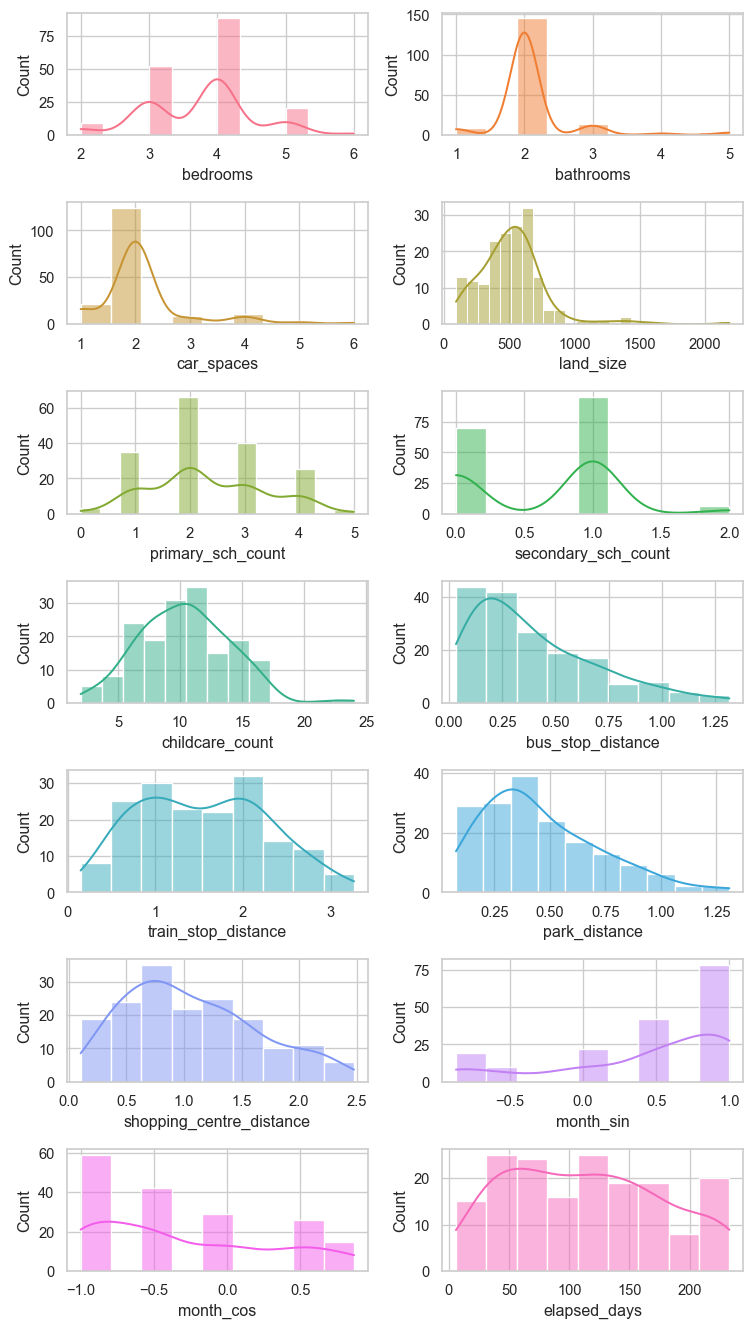

box_fig, axes = plt.subplots(7, 2, figsize = (8, 14))
axes = axes.flatten()

for i, col in enumerate(num_feat):
    sns.boxplot(data = re_data_df[col], ax = axes[i], color=custom_palette[i])

plt.tight_layout()
plt.savefig("images/num_boxplots.png")
plt.show()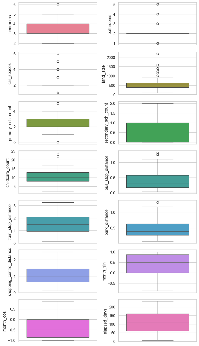

Categorical features

Bar plots of each categorical feature are shown below.

count_fig, axes = plt.subplots(2, 2, figsize = (8, 8))
axes = axes.flatten()

# Plot the categorical data
for i, col in enumerate(cat_feat):
    sns.countplot(x=re_data_df[col], data=re_data_df, hue=re_data_df[col], ax=axes[i], legend=False)

    # Rotate x-axis labels only for the last two plots
    if i in [2, 3]:
        axes[i].tick_params(axis="x", labelrotation=45)

# Remove the unused subplot (12th axis)
for j in range(len(cat_feat), len(axes)):
    count_fig.delaxes(axes[j])

plt.tight_layout()
plt.savefig("images/cat_barplots.png")
plt.show()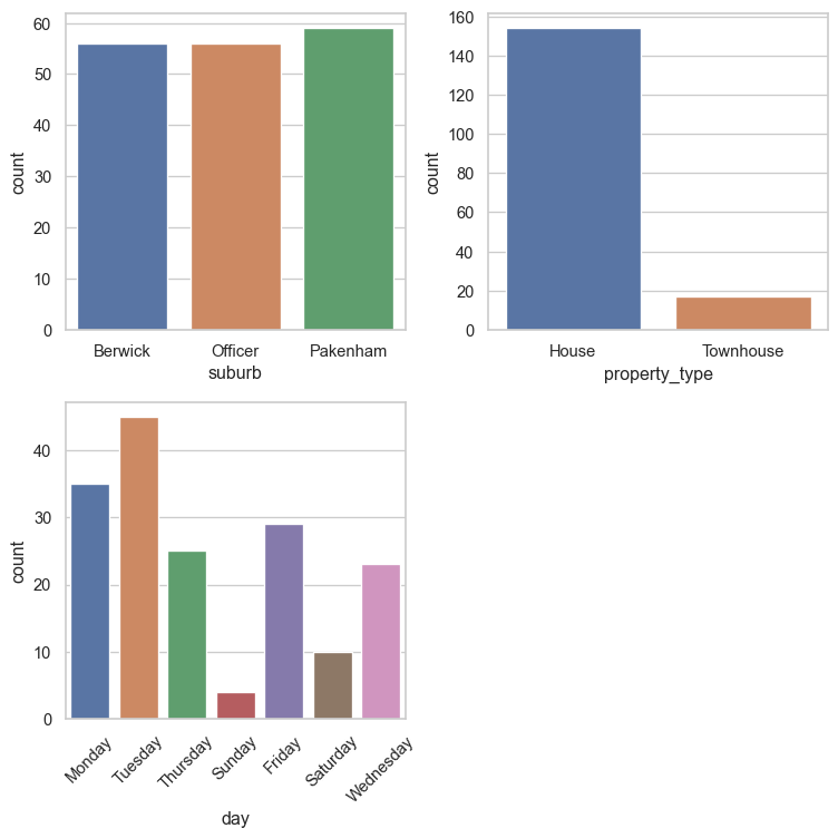

Distribution of property prices

# Distribution of house prices
plt.figure(figsize=(10, 6))

sns.histplot(data=re_data_df, x="sold_price", hue="property_type", bins=30, kde=True,)

# Add vertical lines at the median sold price for each property type
palette = sns.color_palette()
for i, prop_type in enumerate(re_data_df["property_type"].unique()):
    median_price = re_data_df.loc[re_data_df["property_type"] == prop_type, "sold_price"].median()
    plt.axvline(median_price, linestyle="--", label=f"{prop_type} Median", linewidth=2, color=palette[i])

# Format x-axis labels to show values in hundreds of thousands
hist_ax = plt.gca()
hist_ax.xaxis.set_major_formatter(
    ticker.FuncFormatter(lambda price, _: f"{int(price / 1000):,}K")
)

plt.title("Distribution of Property Prices")
plt.xlabel("Sold Price ($)")
plt.ylabel("Frequency")
plt.legend()
plt.tight_layout()
plt.savefig("images/property_price_distribution.png")
plt.show()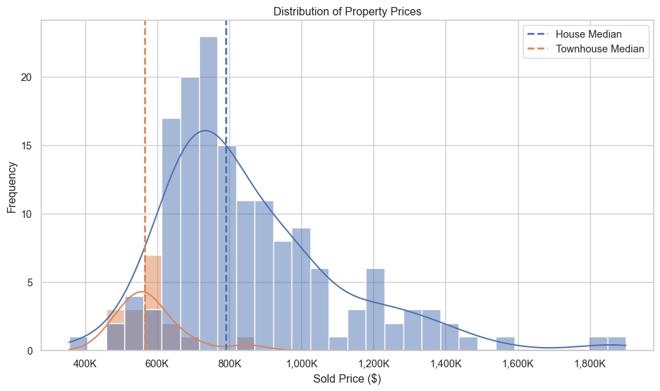

# Distribution of property prices

# Create subplots: 3 rows, 1 column, sharing x and y axes
suburbs = re_data_df["suburb"].unique()
fig, axes = plt.subplots(nrows=3, ncols=1, figsize=(10, 12), sharex=True, sharey=True)

# Define colour palette
palette = sns.color_palette()

# Plot histogram for each suburb in its respective subplot
for i, suburb in enumerate(suburbs):
    ax = axes[i]
    sns.histplot(data=re_data_df[re_data_df["suburb"] == suburb], x="sold_price",
                 bins=30, kde=True, ax=ax, color=palette[i])

    # Add vertical line for median sold price
    median_price = re_data_df.loc[re_data_df["suburb"] == suburb, "sold_price"].median()
    ax.axvline(median_price, linestyle="--", label=f"{suburb} Median", linewidth=2, color=palette[i])

    # Add title and legend
    ax.set_title(f"{suburb}")
    ax.legend()

# Format x-axis labels to show values in thousands
axes[-1].xaxis.set_major_formatter(ticker.FuncFormatter(lambda price, _: f"{int(price/1000):,}K"))

# Set common labels
fig.suptitle("Distribution of Property Prices by Suburb", fontsize=16)
fig.text(0.5, 0.04, "Sold Price ($)", ha='center')
fig.text(0.04, 0.5, "Frequency", va='center', rotation='vertical')
plt.tight_layout(rect=[0.05, 0.05, 1, 0.95])
plt.savefig("images/property_price_distribution_by_suburb.png")
plt.show()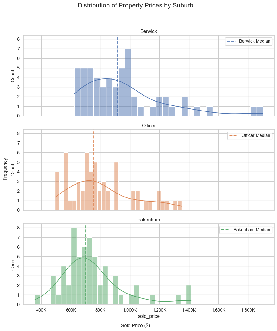

Price trends over time

# Group by month and property_type to calculate average sold_price
price_trends =  red_geo_sch_cc_pt_df.groupby(["month", "property_type"],
                                   observed=False)["sold_price"].mean().reset_index()

# Sort months in calendar order
month_order = ["January", "February", "March", "April", "May", "June", "July", "August"]
price_trends["month"] = pd.Categorical(price_trends["month"], categories=month_order, ordered=True)
price_trends = price_trends.sort_values("month")

# Plotting
ln_fig, ln_ax = plt.subplots(figsize=(10, 6))
sns.lineplot(data=price_trends, x="month", y="sold_price", hue="property_type", marker="o",ax=ln_ax)
ln_ax.set_title("Mean Property Price Trends Over Time by Property Type")
ln_ax.set_xlabel("Month")
ln_ax.set_ylabel("Mean Sold Price ($)")

# Format y-axis labels to show values in hundreds of thousands
ln_ax.yaxis.set_major_formatter(ticker.FuncFormatter(lambda y, _: f"{int(y/1000):,}K"))
plt.xticks(rotation=45)
plt.tight_layout()
plt.savefig("images/price_trends_by_month.png")
plt.show()

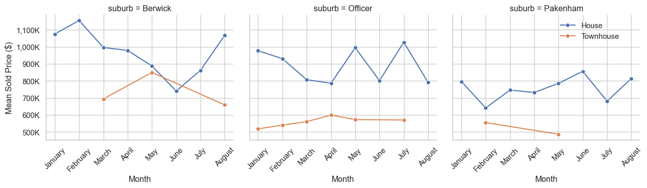
# Set up the plot
g = sns.FacetGrid(red_geo_sch_cc_pt_df, col="suburb", col_wrap=3, height=4, sharey=True)
red_geo_sch_cc_pt_df["month"] = pd.Categorical(red_geo_sch_cc_pt_df["month"], categories=month_order, ordered=True)
g.map_dataframe(
    sns.lineplot,
    x="month",
    y="sold_price",
    hue="property_type",
    marker="o",
    errorbar=None,
)
g.set_axis_labels("Month", "Mean Sold Price ($)")
g.add_legend()
sns.move_legend(g, "upper left", bbox_to_anchor=(0.85, 0.9))

# Rotate x-axis labels for clarity
for g_ax in g.axes.flatten():
    g_ax.yaxis.set_major_formatter(ticker.FuncFormatter(lambda price, _: f"{int(price/1000):,}K"))
    for x_label in g_ax.get_xticklabels():
        x_label.set_rotation(45)

plt.tight_layout()
plt.savefig("images/price_trends_by_suburb.png")
plt.show()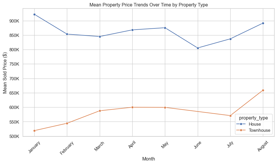

Feature vs target scatter plots for numerical features

# Number of features
num_features = len(num_feat)

# Determine the number of rows needed for 2 columns
num_rows = (num_features + 1) // 2

# Create a figure with subplots
sp_fig, axes = plt.subplots(num_rows, 2, figsize=(16, 5 * num_rows))
axes = axes.flatten()  # Flatten the axes array for easy indexing

# Plot each feature
for i, feature in enumerate(num_feat):
    sp_ax = axes[i]
    sns.scatterplot(x=re_data_df[feature], y=re_data_df["sold_price"], ax=sp_ax)
    sp_ax.set_title(f"{feature} vs Sold Price", fontsize=18)
    sp_ax.set_xlabel(feature, fontsize=18)
    sp_ax.set_ylabel("Sold Price ($)", fontsize=18)
    sp_ax.tick_params(axis='y', labelsize=16)
    sp_ax.tick_params(axis='x', labelsize=16)

    sp_ax.yaxis.set_major_formatter(
        ticker.FuncFormatter(lambda price, _: f"{int(price / 1000):,}K")
    )
    # Calculate correlation coefficient
    corr_coef = re_data_df[feature].corr(re_data_df["sold_price"])

    # Add text box with correlation coefficient
    textstr = f"Correlation: {corr_coef:.2f}"
    bbox_props = dict(boxstyle="round", facecolor="white", alpha=1)
    sp_ax.text(0.05, 0.95, textstr, transform=sp_ax.transAxes, fontsize=18,
            verticalalignment="top", bbox=bbox_props)


# Hide any unused subplots
for j in range(len(num_feat) + 1, len(axes)):
    sp_fig.delaxes(axes[j])

# Adjust layout and save the figure
plt.tight_layout()
plt.savefig("images/features_vs_sold_price.png")
plt.show()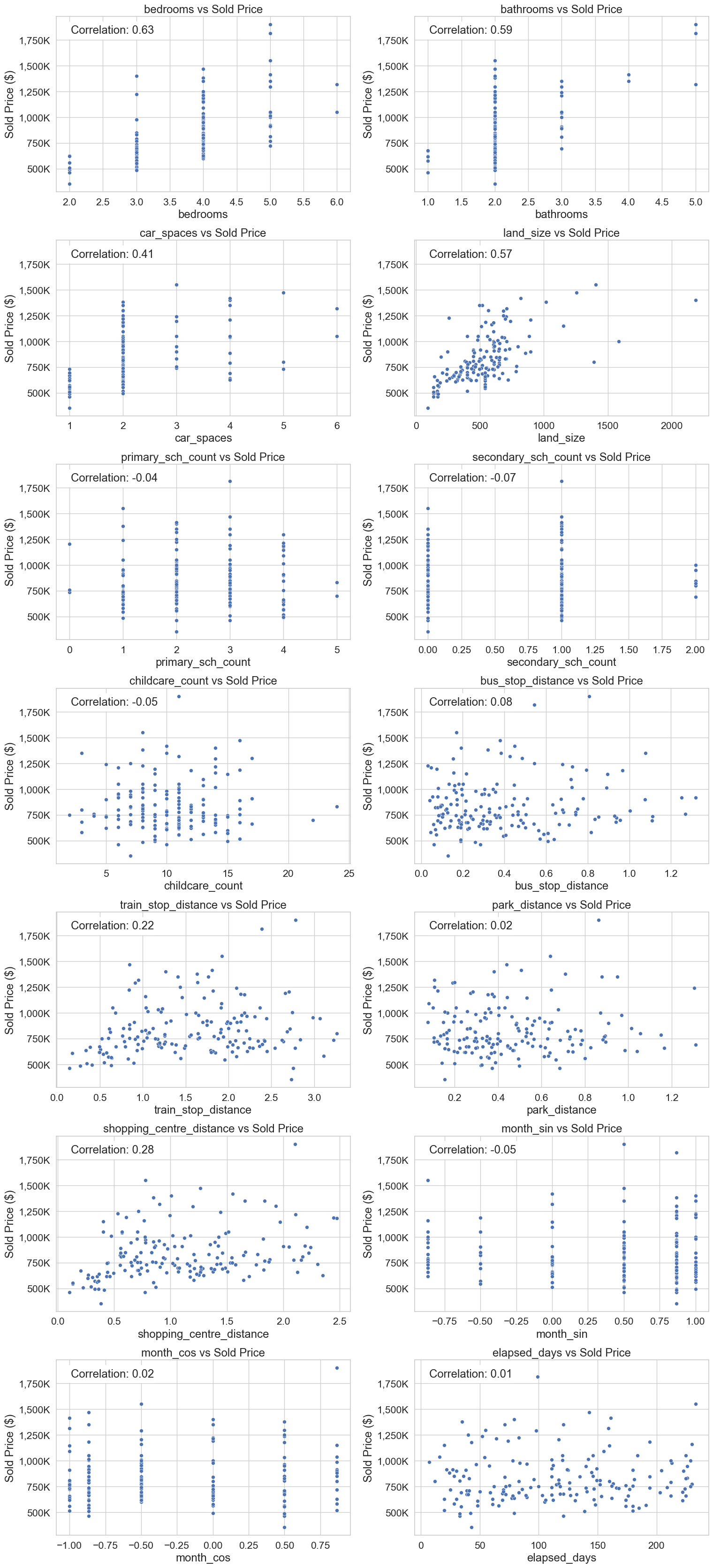

Split data into test and train

An 80/20 split has been used, were 80% of the data is used from training and 20% for testing.

Create features and target

# Define column lists
numerical_cols = num_feat.tolist()
categorical_cols = cat_feat.tolist()

X_df = re_data_df.drop(["sold_price"], axis=1)

# Arrange to have numerical features fist, then categorical features
X_df = X_df[numerical_cols + categorical_cols]

y_df = re_data_df["sold_price"]

print(f"Training shape: {X_df.shape}")
print(f"Target shape: {y_df.shape}")

# Split data into training and test sets
X_train, X_test, y_train, y_test = train_test_split(X_df, y_df, test_size=0.2, random_state=42)

Training shape: (171, 17)
Target shape: (171,)

Encoding and Feature scaling

For consistent workflow, these steps are performed in a pipeline that is configured an executed in the model development sections.

There are no ordinal categorical features, only nominal. Therefore, each categorical feature is encoded using One-Hot encoding. The dummy variables created with One-Hot encoding can create multicollinearity between the dummy variables. This can cause trouble for some regression models and therefore, when appropriate for the model, the first dummy variable for each category is dropped.

The numerical features are all scaled with the robust scaler due to the presence of outliers and skewness in some features.

Model development

This task required at least three regression models to be created. The models used in this work are ElasticNet (linear regression), KNN and Random forrest. ElasticNet and KNN can suffer when there are highly correlated features. The figure below shows a correlation heat map for the features. Cells were the absolute value of the correlation is less than 0.5 have been removed from the plot, highlight which features show some stronger correlation. As there are some highly correlated features, it was decided to drop the first dummy feature of One-Hot encoding

# Create the ColumnTransformer
preprocessor = ColumnTransformer([
    ("num", StandardScaler(), numerical_cols),
    ("cat", OneHotEncoder(handle_unknown="ignore"), categorical_cols)
])

# Create a pipeline with only the preprocessing step
preprocess_pipeline = Pipeline([
    ("preprocess", preprocessor)
])

# Fit and transform the data
transformed_data = preprocess_pipeline.fit_transform(X_train)

# Get feature names for the transformed data
encoded_feature_names = preprocess_pipeline.named_steps["preprocess"].named_transformers_["cat"].get_feature_names_out(categorical_cols)
all_feature_names = numerical_cols + list(encoded_feature_names)

# Convert the transformed data to a DataFrame
transformed_df = pd.DataFrame(transformed_data.toarray() if hasattr(transformed_data, "toarray") else transformed_data,
                              columns=all_feature_names)

# Compute the correlation matrix
corr_matrix = transformed_df.corr()

# Set the threshold for highlighting
threshold = 0.5

# Create a mask for values below the threshold
mask = abs(corr_matrix) < threshold

# Set up the matplotlib figure
plt.figure(figsize=(10, 8))

# Generate a heatmap using seaborn
sns.heatmap(
    corr_matrix,
    mask=mask,
    annot=False,
    cmap="coolwarm",
    linewidths=0.5,
    vmin=-1,
    vmax=1,
)

# Add title
plt.title("Feature Correlation Matrix Heatmap")

# Save the heatmap to a file
plt.tight_layout()
plt.savefig("images/lr_correlation_heatmap.png")
plt.show()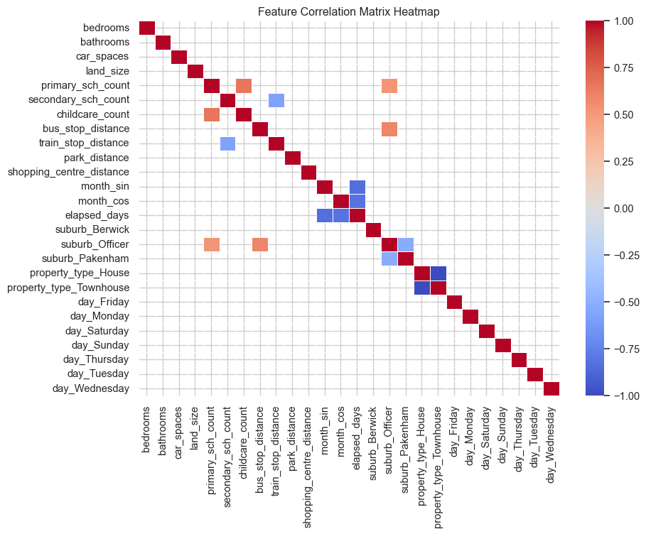

def evaluate_model_learningcurves(best_pipeline, X, y, label=None, n_folds=10):
    """
    Function to plot learning curves

    :param best_pipeline: regression pipeline instance
    :param X: feature matrix
    :param y: target vector
    :param label: plot label
    :param n_folds: number of cross-validation folds (default is 5)
    :returns: None
    """
    # Generate learning curve data
    train_sizes, train_scores, test_scores = learning_curve(
        best_pipeline,
        X,
        y,
        cv=n_folds,
        scoring="neg_mean_absolute_error",
        train_sizes=np.linspace(0.1, 1.0, 10),
        n_jobs=-1,
    )

    # Calculate mean and standard deviation
    train_scores_mean = -np.mean(train_scores, axis=1)
    test_scores_mean = -np.mean(test_scores, axis=1)
    train_scores_std = -np.std(train_scores, axis=1)
    test_scores_std = -np.std(test_scores, axis=1)

    # Plot the learning curve
    plt.figure(figsize=(10, 6))
    plt.title(f"Learning Curve for {label}")
    plt.xlabel("Training Set Size")
    plt.ylabel("MAE")
    plt.grid(True)

    # Plot with shaded standard deviation
    plt.fill_between(
        train_sizes,
        train_scores_mean - train_scores_std,
        train_scores_mean + train_scores_std,
        alpha=0.1,
        color="r",
    )
    plt.fill_between(train_sizes, test_scores_mean - test_scores_std,
                     test_scores_mean + test_scores_std, alpha=0.1, color="g")

    plt.plot(train_sizes, train_scores_mean, 'o-', color="r", label="Training score")
    plt.plot(train_sizes, test_scores_mean, 'o-', color="g", label="Cross-validation score")

    plt.legend(loc="best")
    plt.tight_layout()
    # Save the figure
    plt.savefig(f"images/{label}_learning_curve.png")
    plt.show()

def evaluate_model_cv(best_pipeline, X, y, label=None, n_folds=10):
    """
    Perform cross-validation on a regression model and plot metrics across folds.

    :param best_pipeline: regression pipeline instance
    :param X: feature matrix
    :param y: target vector
    :param label: plot label
    :param n_folds: number of cross-validation folds (default is 5)
    :returns: None
    """
    # Perform cross-validation
    scores = cross_validate(
        best_pipeline,
        X,
        y,
        cv=n_folds,
        scoring=["neg_mean_absolute_error"],
        return_train_score=True,
    )

    # Extract and convert negative scores to positive
    mae_test_scores = -scores["test_neg_mean_absolute_error"]
    mae_train_scores = -scores["train_neg_mean_absolute_error"]

    # Create fold indices
    folds = np.arange(1, n_folds + 1)

    # Plot metrics across folds
    fig, ax = plt.subplots(figsize=(10, 6))

    ax.set_xlabel("Fold")
    ax.set_ylabel("MAE", color="black")
    ax.plot(folds, mae_test_scores, marker="s", label="Cross-validation scores", color="tab:green")
    ax.plot(folds, mae_train_scores, marker="s", label="Training scores", color="tab:red")
    ax.tick_params(axis="y", labelcolor="black")


    # Combine legends from both axes
    lines_1, labels_1 = ax.get_legend_handles_labels()
    ax.legend(lines_1, labels_1, loc="upper right")

    plt.title("Cross-Validation Metric per Fold")
    plt.tight_layout()
    plt.savefig(f"images/{label}_cv_metrics_plot.png")
    plt.show()

def print_test_metrics(model, data):
    """
    Function to print metrics for test set for a given model

    :param model: Name of the model
    :param data: Results DataFrame
    :return: None
    """
    # Print the table with model name as header
    print(f"{model} performance on Test set:")

    # Print headers
    for key in data[model]:
        print(f"{key:<15}", end="")  # Adjust spacing as needed
    print()

    # Print values
    for value in data[model].values():
        print(f"{value:<15}", end="")
    print()

# Dictionary to store results from each model
model_results={}

# Dictionary to store the best models for each type
best_models = {}

Model1: ElasticNet

ElasticNet has been chosen to balance Ridge and Lasso regularisation and provide some feature selection.

Hyperparameter tuning

The ElasticNet model combines both L1 (Lasso) and L2 (Ridge) regularisation, and it has a few key hyperparameters that control how it behaves. The two #parameter that have been adjusted in this work are:

alpha: Controls the overall strength of regularisation.

• Higher values → more regularisation (simpler model, possibly under-fitting).
• Lower values → less regularisation (more complex model, possibly over-fitting).

l1_ratio: Controls the mix between L1 and L2 regularisation:

• l1_ratio = 0 → pure Ridge (L2)
• l1_ratio = 1 → pure Lasso (L1)
• 0 < l1_ratio < 1 → ElasticNet mix

# Create the full pipeline
pipeline_en = Pipeline(steps=[
    ("preprocessor", preprocessor),
    ("model", ElasticNet(max_iter=10000, random_state=42))
])

# Define hyperparameter grid
param_grid_en = {"model__alpha": [0.1, 1.0, 10.0], "model__l1_ratio": [0.1, 0.5, 0.9, 0.95]}

# Set up GridSearchCV
grid_search_en = GridSearchCV(
    pipeline_en,
    param_grid_en,
    cv=10,
    scoring="neg_mean_absolute_error",
    n_jobs=-1
)

# Fit the model
grid_search_en.fit(X_train, y_train)

# Predict and evaluate on test set
y_pred = grid_search_en.predict(X_test)
r2 = r2_score(y_test, y_pred)
rmse = root_mean_squared_error(y_test, y_pred)
mae = mean_absolute_error(y_test, y_pred)

# Store ElasticNet results
model_results["ElasticNet"] = {
    "R2 Score": round(r2, 3),
    "MAE": round(mae, 2),
    "RMSE": round(rmse, 2),
}

# Store the best estimator
best_models["ElasticNet"] = grid_search_en.best_estimator_

# Output the best parameters and score
print("Best parameters:", grid_search_en.best_params_)
print(f"Best Validation Score (MAE): {-grid_search_en.best_score_:.2f}")

Best parameters: {'model__alpha': 1.0, 'model__l1_ratio': 0.9}
Best Validation Score (MAE): 107308.94

evaluate_model_learningcurves(grid_search_en.best_estimator_, X_train, y_train, label="ElasticNet")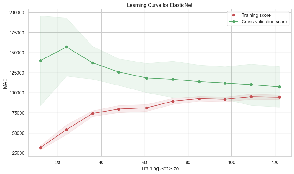

evaluate_model_cv(grid_search_en.best_estimator_, X_train, y_train, label="lr")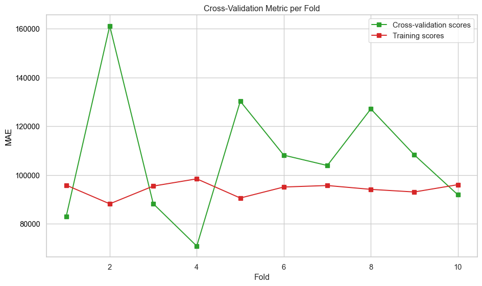

print_test_metrics("ElasticNet", model_results)

ElasticNet performance on Test set:
R2 Score       MAE            RMSE           
0.77           79649.33       106277.19      

kNN

This section builds kNN model. KNN was chosen for the second model for the following reasons:

• Non-parametric and flexible: kNN doesn’t assume any underlying distribution or functional form (like linear regression does). This is useful when property prices depend on complex, non-linear relationships (e.g., location, amenities, number of schools).

• Intuitive and easy to understand: kNN predicts a house price by averaging the prices of the “k” most similar houses.

Hyperparameter tuning

kNN has several hyperparameters

n_neighbors (k): Sets the number of neighbours to consider when making a prediction.

• Small k → more sensitive to noise, lower bias, higher variance.
• Large k → smoother predictions, higher bias, lower variance.

weights: How the neighbours contribute to the value.

• uniform: All neighbours contribute equally.
• distance: Closer neighbours have more influence.

metric: Defines how distance is calculated between points.

# Create the full pipeline
# Dropping dummies in one-hot made the performance worse.
pipeline_knn = Pipeline(steps=[
    ("preprocessor", preprocessor),
    ("model", KNeighborsRegressor())
])

# Define K range to search
n_samples = len(X_train)
sqrt_n = int(np.sqrt(n_samples))

# Test around this value
k_range = list(range(1, min(sqrt_n * 2, 50)))

param_grid_knn = {
    "model__n_neighbors": k_range,
    "model__weights": ["uniform", "distance"],
    "model__metric": ["euclidean", "manhattan", "chebyshev", "minkowski"],
    "model__p": [1, 2]  # Only used when metric is 'minkowski'
}

# kNN grid search with CV
knn_grid_search = GridSearchCV(
    pipeline_knn,
    param_grid_knn,
    cv=10,
    scoring="neg_mean_absolute_error",
    n_jobs=-1
)

knn_grid_search.fit(X_train, y_train)

# Predict and evaluate on test set
y_pred = knn_grid_search.predict(X_test)
r2 = r2_score(y_test, y_pred)
rmse = root_mean_squared_error(y_test, y_pred)
mae= mean_absolute_error(y_test, y_pred)

# Store KNN results
model_results["kNN"] = {
    "R2 Score": round(r2, 3),
    "MAE": round(mae, 2),
    "RMSE": round(rmse, 2),
}

# Store the best kNN model
best_models["kNN"] = knn_grid_search.best_estimator_

print(f"Best k: {knn_grid_search.best_params_}")
print(f"Best Validation Score (MAE): {-knn_grid_search.best_score_:.4f}")

Best k: {'model__metric': 'euclidean', 'model__n_neighbors': 4, 'model__p': 1, 'model__weights': 'distance'}
Best Validation Score (MAE): 127873.1405

# Calculate the error versus k value
k_scores = []
for k in k_range:
    pipeline = Pipeline([
        ("preprocessor", preprocessor),
        ("model", KNeighborsRegressor(n_neighbors=k, weights="distance",
                                      metric="euclidean"))
    ])
    cv_scores = cross_val_score(pipeline, X_train, y_train, cv=10, scoring="neg_mean_absolute_error")
    k_scores.append(-cv_scores.mean())

plt.plot(k_range, k_scores)
plt.xlabel("k")
plt.ylabel("MAE")
plt.title("MAE vs k")
plt.tight_layout()
plt.savefig("images/rmse_vs_k.png")
plt.show()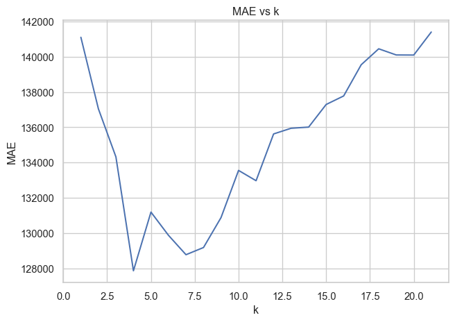

evaluate_model_learningcurves(knn_grid_search.best_estimator_, X_train, y_train, label="kNN")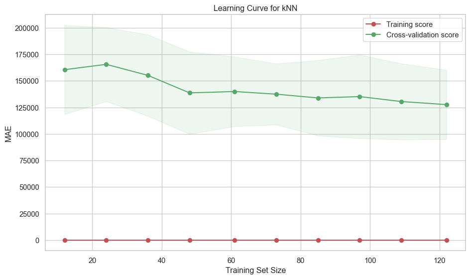

evaluate_model_cv(knn_grid_search.best_estimator_, X_train, y_train, label="knn")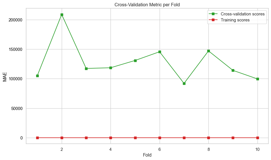

print_test_metrics("kNN", model_results)

kNN performance on Test set:
R2 Score       MAE            RMSE           
0.633          100021.53      134346.81      

Random Forrest

This section builds a random forest model. Reasons for selecting Random Forest:

• Unlike linear models (e.g., ElasticNet), Random Forest can model complex interactions between features without needing to explicitly define them.

• Each tree is trained on a random subset of the data, so outliers have less influence on the overall prediction.

• Feature importance insights: Provides estimates of feature importance.

• Good generalisation: Averaging predictions across many trees reduces over-fitting compared to a single decision tree.

Hyperparameter tuning

The scikit learn Random Forest regressor has many hyperparameters. However, most of these relate to the underlying decision trees and those settings are concerned with pre-pruning controls. For the Random Forest model in this work, fully grown trees are used, which means that the hyperparameters relating to the decision trees can be left at their default values (no pre-pruning) and only those parameters affecting the random forest algorithm are changes. Those parameters are:

n_estimators: Number of trees in the forest.

• More trees generally improve performance but increase training time.
• Too many trees might lead to over-fitting.

criterion: The function to measure the quality of a split.

max_features: The number of features to take into account in order to make the best split.

# Create the full pipeline
pipeline_rf = Pipeline(
    steps=[
        ("preprocessor", preprocessor),
        ("model", RandomForestRegressor(random_state=42)),
    ]
)

param_grid_rf = {
    "model__n_estimators": [100, 200, 400, 500, 600,800],
    "model__criterion": ["squared_error", "absolute_error", "friedman_mse", "poisson"],
    "model__max_features": ["sqrt", "log2", None],
}

# Random forest grid search with CV
rf_grid_search = GridSearchCV(
    pipeline_rf,
    param_grid_rf,
    cv=10,
    scoring="neg_mean_absolute_error",
    n_jobs=-1,
)

rf_grid_search.fit(X_train, y_train)

# Predict and evaluate on test set
y_pred = rf_grid_search.predict(X_test)
r2 = r2_score(y_test, y_pred)
rmse = root_mean_squared_error(y_test, y_pred)
mae = mean_absolute_error(y_test, y_pred)

# Store results
model_results["Random Forest"] = {
    "R2 Score": round(r2, 3),
    "MAE": round(mae, 2),
    "RMSE": round(rmse, 2),
}

# Store the best random forest
best_models["Random Forest"] = rf_grid_search.best_estimator_

print(f"Best Parameters: {rf_grid_search.best_params_}")
print(f"Best Validation Score (MAE): {-rf_grid_search.best_score_:.4f}")

Best Parameters: {'model__criterion': 'squared_error', 'model__max_features': None, 'model__n_estimators': 600}
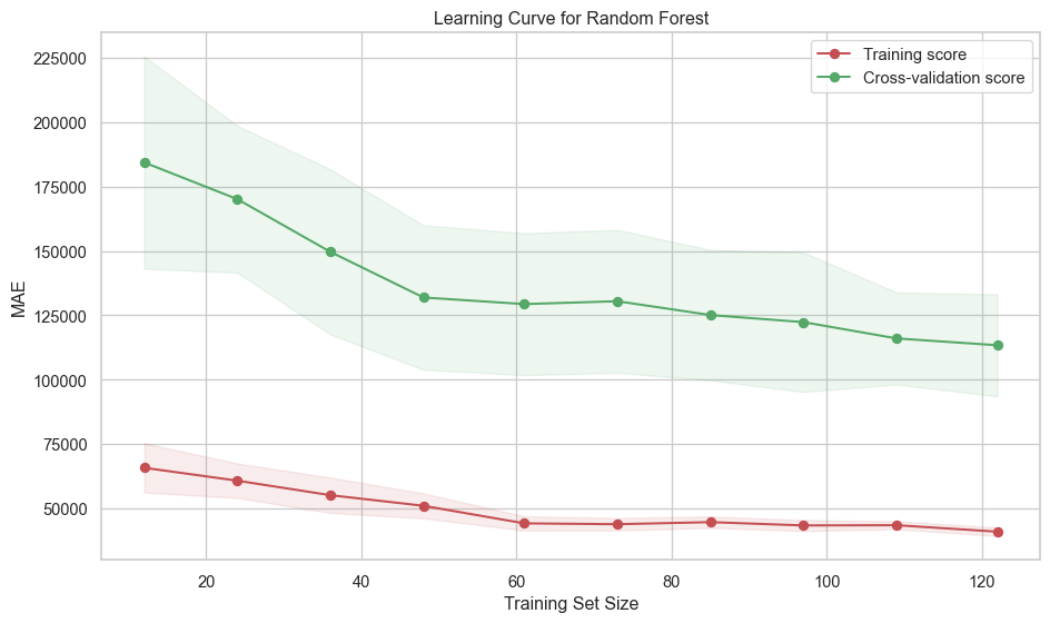
Best Validation Score (MAE): 112635.7592

evaluate_model_learningcurves(
    rf_grid_search.best_estimator_, X_train, y_train, label="Random Forest"
)

evaluate_model_cv(rf_grid_search.best_estimator_, X_train, y_train, label="rf")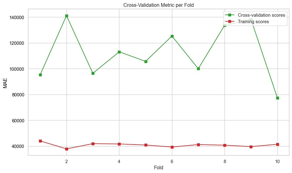

print_test_metrics("Random Forest", model_results)

Random Forest performance on Test set:
R2 Score       MAE            RMSE           
0.699          80013.42       121542.34      

Feature importance

Two methods were used to analyse feature importance model:

• ElasticNet and Random Forest

• Model-Based Importance and SHAP analysis

• kNN

• Permutation importance and SHAP analysis

Model-Based Importance - use inherent attribute of the model to asses feature importance. For ElasticNet, use coefficient magnitudes and for Random Forest use the Mean Decrease in Impurity (MDI).

Permutation importance - evaluates how much a model’s performance decreases when a feature’s values are randomly shuffled. If shuffling a feature significantly worsens the model’s performance, that feature is considered important.

SHAP analysis - ensures robust statistical inference by examining feature contributions at both individual and aggregate levels, while accounting for potential non-linear effects and class-specific patterns in the data.

For reporting the Model-base and permutation importances have been grouped together and the SHAP values are reported together.

# Dictionary to store feature importances
feature_importances = {}

# Transform the train/test data
X_train_transformed = preprocessor.transform(X_train)
X_test_transformed = preprocessor.transform(X_test)

# Dictionary to store SHAP values
shap_data = {}

for name, best_pipe in best_models.items():
    best_pipe.fit(X_train, y_train)

    # Get feature names after preprocessing
    feature_names = best_pipe.named_steps["preprocessor"].get_feature_names_out()
    feature_names = [name.split("__")[-1] for name in feature_names]

    model = best_pipe.named_steps["model"]

    if name == "Random Forest":
        # Get feature importances from model
        importances = model.feature_importances_

        # Use TreeExplainer for RandomForest
        explainer = shap.TreeExplainer(model)
        shap_values = explainer.shap_values(X_test_transformed)

    elif name=="ElasticNet":
        # Get coefficients from the ElasticNet model and normalise coefficients
        importances = np.abs(model.coef_)

        explainer = shap.Explainer(model, X_test_transformed, feature_names=feature_names)
        shap_values = explainer(X_test_transformed).values

    else: # kNN
        result = permutation_importance(best_pipe, X_test, y_test, n_repeats=10, random_state=42)
        importances = result.importances_mean

        # Use SHAP KernelExplainer for kNN
        explainer = shap.KernelExplainer(model.predict, X_train_transformed)
        shap_values = explainer.shap_values(X_test_transformed)

    # Store features
    features_imp = sorted(zip(feature_names, importances), key=lambda x: x[1], reverse=True)
    feature_importances[name] = dict(features_imp)

    # Compute mean absolute SHAP values
    mean_shap_values = np.abs(shap_values).mean(axis=0)
    features_shap = sorted(zip(feature_names, mean_shap_values), key=lambda x: x[1], reverse=True)
    shap_data[name] = dict(features_shap)

# Create summary table
importances_df = pd.DataFrame(feature_importances).fillna(0)
importances_df.head()

# Sort the DataFrame by the first column in descending order
sorted_index = importances_df["ElasticNet"].sort_values(ascending=False).index
df_sorted_importances = importances_df.loc[sorted_index]

# Create summary table
shap_df = pd.DataFrame(shap_data).fillna(0)

# Sort the DataFrame by the first column in descending order
sorted_index = shap_df["ElasticNet"].sort_values(ascending=False).index
df_sorted_shap = shap_df.loc[sorted_index]

Using 136 background data samples could cause slower run times. Consider using shap.sample(data, K) or shap.kmeans(data, K) to summarize the background as K samples.

# Group 1 - permutation and model-based importances

# Set up the figure and axes for feature importance plot
fig, axes = plt.subplots(nrows=1, ncols=3, figsize=(15, 8), sharey=True)

# Define colour palettes
palettes = ["Blues_d", "Greens_d", "Reds_d"]

# Plot each chart
for i, col in enumerate(df_sorted_importances.columns):
    sns.barplot(x=df_sorted_importances[col], y=df_sorted_importances.index, ax=axes[i], palette=palettes[i],
                hue=df_sorted_importances.index, legend=False)
    axes[i].set_title(col, fontsize=18)
    axes[i].set_xlabel("Importance", fontsize=18)
    axes[i].set_ylabel("Feature" if i == 0 else "", fontsize=18)
    axes[i].tick_params(axis='y', labelsize=16)
    axes[i].tick_params(axis='x', labelsize=16)

# Adjust layout and save the figure
plt.tight_layout()
plt.savefig("images/feature_importance_grp1.png")
plt.show()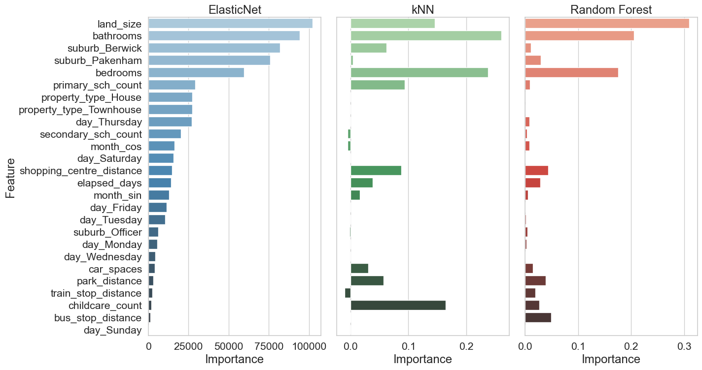

# Group 2 - SHAP values

# Set up the figure and axes
fig, axes = plt.subplots(nrows=1, ncols=3, figsize=(15, 8), sharey=True)

# Define colour palettes
palettes = ["Blues_d", "Greens_d", "Reds_d"]

# Plot each chart
for i, col in enumerate(df_sorted_shap.columns):
    sns.barplot(x=df_sorted_shap[col], y=df_sorted_shap.index, ax=axes[i], palette=palettes[i],
                hue=df_sorted_shap.index, legend=False)
    axes[i].set_title(col, fontsize=18)
    axes[i].set_xlabel("Absolute Mean SHAP Value", fontsize=18)
    axes[i].set_ylabel("Feature" if i == 0 else "", fontsize=18)
    axes[i].tick_params(axis='y', labelsize=16)
    axes[i].tick_params(axis='x', labelsize=16)
# Adjust layout and save the figure
plt.tight_layout()
plt.savefig("images/feature_importance_grp2.png")
plt.show()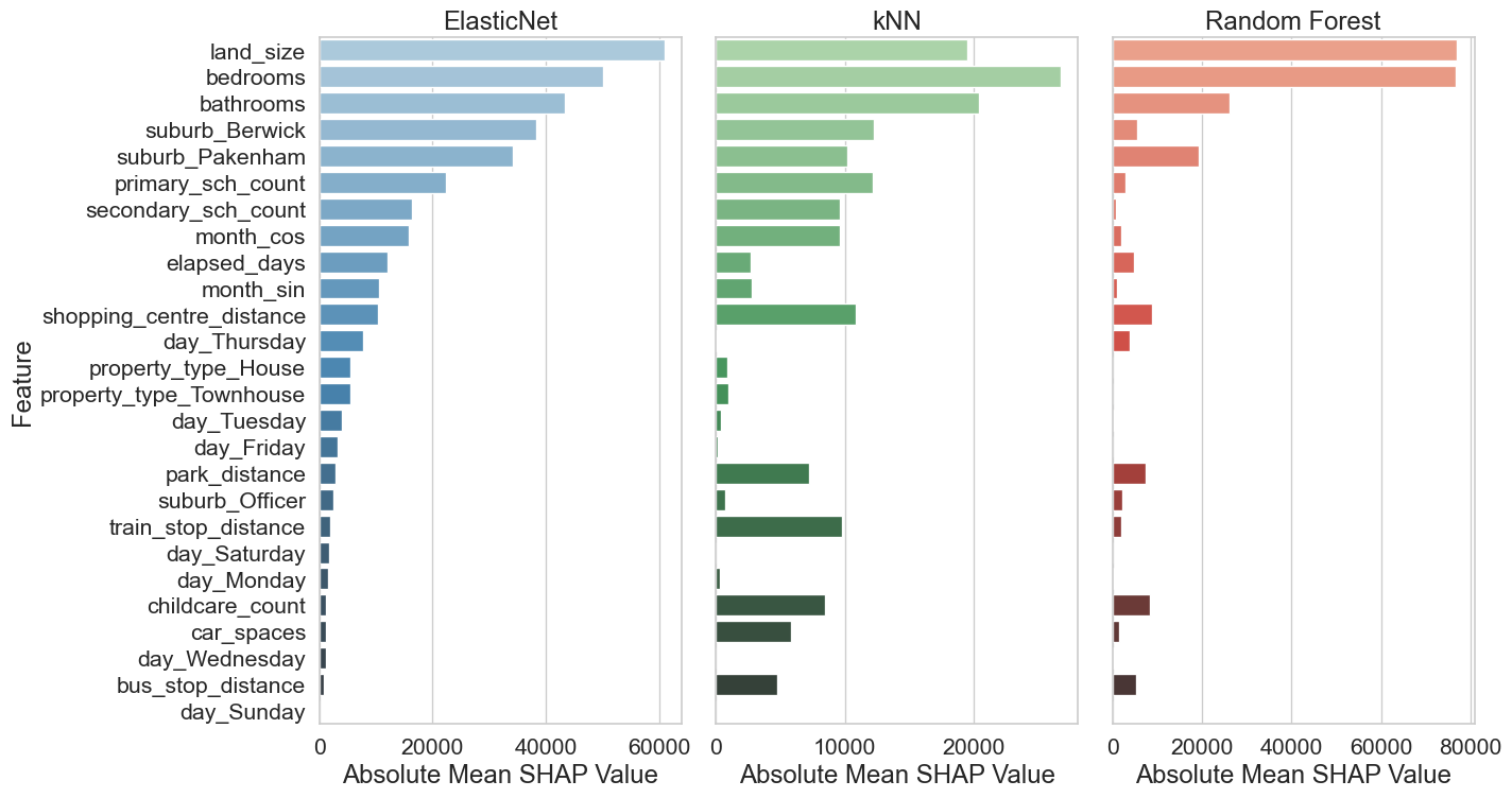

Recommended model

The figure below shows the comparison of the MAE, RMSE and \(R^2\) metrics for each model. The ElasticNet model has the highest \(R^2\) and lowest RMSE. Its MAE is slightly higher than Random Forest which has the lowest value for this metric. The kNN model has the worst of all three metrics. Based on these metrics, ElasticNet is the recommended model.

# Model names
models = ["ElasticNet", "kNN", "Random Forest"]

# R² scores, RMSE values, and MAE values
r2_scores = [metrics["R2 Score"] for metrics in model_results.values()]
mae_values = [metrics["MAE"] for metrics in model_results.values()]
rmse_values = [metrics["RMSE"] for metrics in model_results.values()]

# Set the positions and width for the bars
bar_x = np.arange(len(models))
width = 0.35

# Create the figure and primary axis
mod_fig, ax1 = plt.subplots(figsize=(10, 6))

# Plot RMSE and MAE on primary y-axis
bars_rmse = ax1.bar(
    bar_x - width / 2, rmse_values, width, label="RMSE", color="lightblue"
)
bars_mae = ax1.bar(bar_x + width / 2, mae_values, width, label="MAE", color="orange")
ax1.set_xlabel("Model")
ax1.set_ylabel("Error Metrics (RMSE & MAE)", color="black")
ax1.tick_params(axis="y", labelcolor="black")
ax1.set_xticks(bar_x)
ax1.set_xticklabels(models)

# Create secondary y-axis for R² scores
ax2 = ax1.twinx()
bars_r2 = ax2.plot(
    bar_x, r2_scores, label="R² Score", color="green", marker="o", linestyle="-"
)
ax2.set_ylabel("R² Score", color="green")
ax2.tick_params(axis="y", labelcolor="green")
ax2.set_ylim(0, 1)

# Add legend
mod_fig.legend(loc="upper center", bbox_to_anchor=(0.75, 0.9), ncol=3)

# Add title
plt.title("Model Performance Comparison")

# Save the plot
plt.tight_layout()
plt.savefig("images/model_performance_comparison.png")

# Show the plot
plt.show()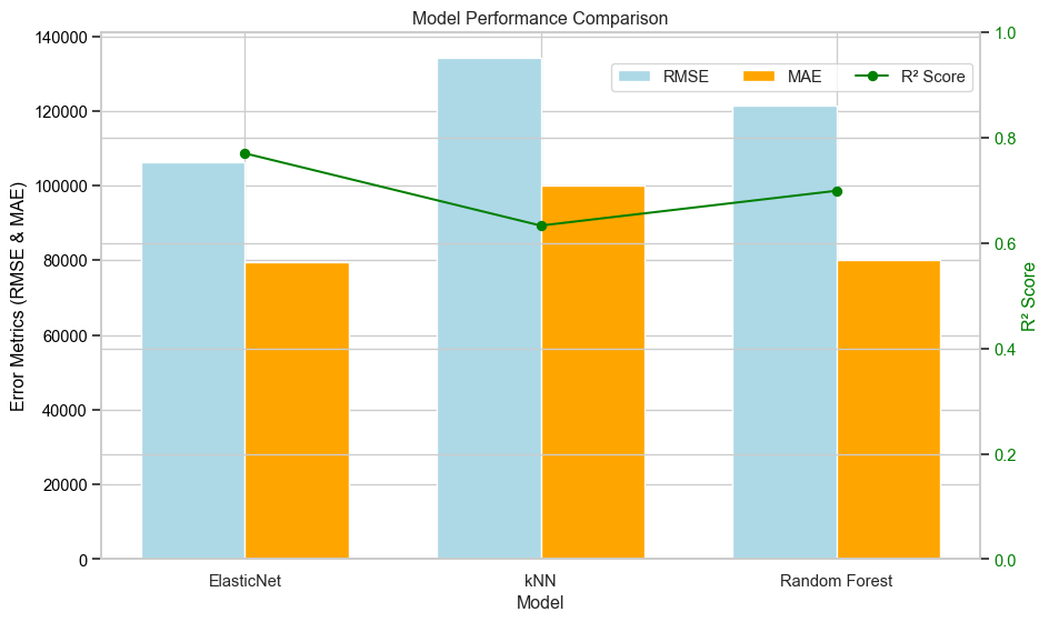

Model Deployment

To delopy the best model, it is first saved to a file so it can be uploaded and utilised in a Streamlit web application. The code for the Streamlit app can be found below and in the GitHub repository at https://github.com/dwstephens/SIT720-T8_2D. To predict the property price using the web application, the user is required to enter the details about the property. These are the features the model was built using. To keep the application simple, the user needs to enter values for most of the engineered features as well, except for those derived from the date. The features derived from the date are calculated in the web application using a custom transformer. Encoding and scaling are performed in the pipeline encapsulated with the loaded model.

The Streamlit web application is hosted on the Streamlit community cloud and can be found at https://sit720-t82d-bdzrxstjm3nmm3v8yashcu.streamlit.app/.

import joblib
# Save the pipeline to a joblib file
joblib.dump(best_models["ElasticNet"], 'property_pipeline.joblib')

['property_pipeline.joblib']