import numpy as np
import pandas as pd
import matplotlib.pyplot as pltWorking with pandas Data Frames (Heterogeneous Data)
Introduction
This task requires working with pandas data frames and Python to conduct a data analysis exercise involving meteorological data for three airports in New York. The meteorological data is loaded into a pandas data frame from a text file. Pandas operations are used to filter and aggregate the data to enable plotting of the mean monthly and daily wind speeds for different airports. Additional analysis is performed for JFK airport to handle missing data and plot the daily average temperature throughout 2013.
Data input
A provided data file nycflights13_weather.csv.gz that contained hourly meteorological data for three airports in New York: EWR, JFK and LGA was used for this analysis. The data contained in the file is:
- origin – weather station: LGA, JFK, or EWR,
- year, month, day, hour – time of recording,
- temp, dewp – temperature and dew point in degrees Fahrenheit,
- humid – relative humidity,
- wind_dir, wind_speed, wind_gust – wind direction (in degrees), speed and gust speed (in mph),
- precip – precipitation, in inches,
- pressure – sea level pressure in millibars,
- visib – visibility in miles,
- time_hour – date and hour (based on the year, month, day, hour fields)
This file is loaded into a pandas data frame using the pd.read_csv function. Any lines containing ‘#’ are ignored when loading. it.
# Load data file in dataframe
nyc_ap_weather = pd.read_csv("nycflights13_weather.csv.gz",comment="#")
Covert all columns so they use SI units
For this step we use the pandas apply method a helper function fahrenheit_to_celsius and lambda functions to do the appropriate conversion for each variable.
# Helper function for temperature conversion
def fahrenheit_to_celsius(fahrenheit):
    """
    This function takes a Fahrenheit value and returns the Celsius equivalent.

    The formula is C = (F-32)* 5/9

    :param fahrenheit: Input temperature in Fahrenheit.
    :return: Temperature in Celsius.
    """
    return (fahrenheit - 32) * 5/9
# Convert "temp" and "dewp" from Fahrenheit to Celsius
nyc_ap_weather["temp"] = nyc_ap_weather["temp"].apply(fahrenheit_to_celsius)
nyc_ap_weather["dewp"] = nyc_ap_weather["dewp"].apply(fahrenheit_to_celsius)
# Convert "precip" to millimetres
nyc_ap_weather["precip"] = nyc_ap_weather["precip"].apply(lambda x:x*25.4)
# Convert "visib" to metres
nyc_ap_weather["visib"] = nyc_ap_weather["visib"].apply(lambda x:x*1609.34)
# Convert "wind_speed" and "wind_gust" to m/s
nyc_ap_weather["wind_speed"] = nyc_ap_weather["wind_speed"].apply(lambda x:x*0.44704)
nyc_ap_weather["wind_gust"] = nyc_ap_weather["wind_gust"].apply(lambda x:x*0.44704)Compute monthly mean wind speeds for all three airports
Before calculating the mean for each airport, we check that the recorded hourly wind speed is not above the highest recorded Hurricane wind speed (96 m/s). Values larger than this are likely to be erroneous and are replaced with NaN so they don’t impact the calculation of the mean.
# Check for any wind speeds above the highest recorded Hurricane (345 km/h | 96 m/s) and replace any found with NaN
nyc_ap_weather.loc[(nyc_ap_weather["wind_speed"] >= 96), "wind_speed"] = np.nan

# Calculate the monthly average wind_speed at all three airports
monthly_ave_wind_speed = nyc_ap_weather.groupby(["origin", "year", "month"])[["wind_speed"]].mean(numeric_only=True).reset_index()
Plot of the monthly mean wind speeds for EWR, JFK and LGA
Now that the monthly mean speed has been calculated for each airport, we can plot these on the same figure for visual comparison.
def plot_monthly_average(months, data, origin, colour, variable="wind_speed"):
    # Create plot of average wind_speed versus date
    plt.plot(months, data[data.origin == origin][variable], label=origin, color=colour)
    plt.xlabel("Month")
    plt.ylabel("Monthly average wind speed [m/s]")

# Create an array of dates, required for the x-axis
month_dates = np.arange("2013-01-01", "2014-01-01", dtype="datetime64[M]")

# Set figure size
plt.figure(figsize=(11, 6))

# Plot LGA
plot_monthly_average(month_dates, monthly_ave_wind_speed, colour="tab:blue", origin="LGA")
# Plot EWR
plot_monthly_average(month_dates, monthly_ave_wind_speed, colour="tab:orange", origin="EWR")
# Plot JFK
plot_monthly_average(month_dates, monthly_ave_wind_speed, colour="tab:green", origin="JFK")

plt.title("Monthly mean wind speeds for NYC airports during 2013")
# Add legend
plt.legend()
plt.show()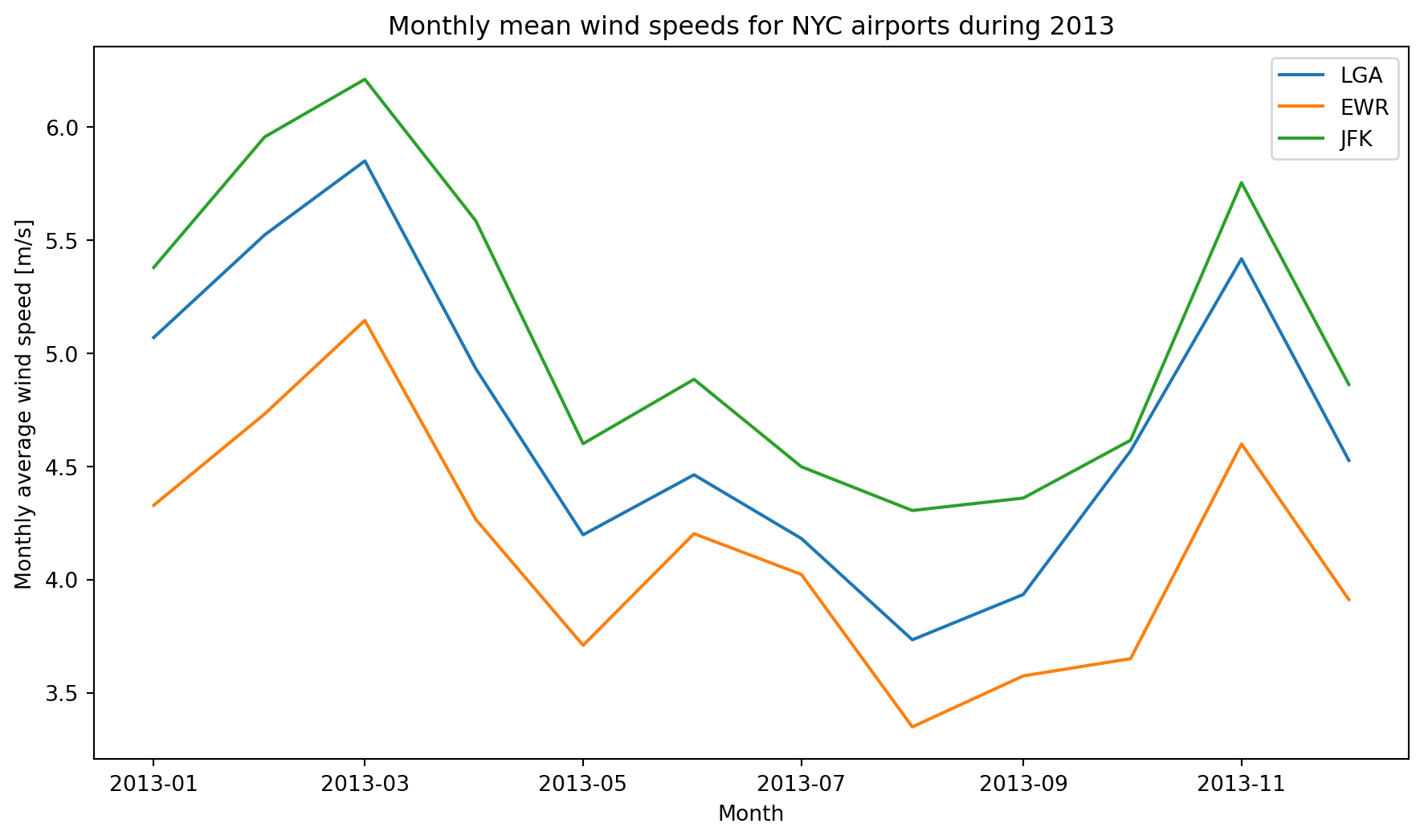
The monthly average wind speed for each airport follows a seasonal pattern with higher average wind speeds in the cooler months and lower monthly average wind speeds in the warmer months. JFK has the highest monthly wind speeds throughout the year, and EWR has the lowest.
Compute daily mean wind speed for LGA airport
We filter the data frame on origin == “LGA”, then group by “year”, “month”, and “day”, select only the “wind_speed” column and call the mean function.
# Calculate the daily average wind_speed at LGA
daily_ave_wind_speed = nyc_ap_weather[nyc_ap_weather.origin=="LGA"].groupby(["year","month","day"])[["wind_speed"]].mean(numeric_only=True).reset_index()
Plot of daily mean wind speeds at LGA
# Create an array of dates, required for the x-axis
dates = np.arange("2013-01-01", "2013-12-31", dtype="datetime64[D]")

# Set figure size
plt.figure(figsize=(11, 6))

# Create line plot of daily average wind_speed
plt.plot(dates, daily_ave_wind_speed["wind_speed"], color="black")
plt.xlabel("Month")
plt.ylabel("Daily average wind speed [m/s] at LGA")
plt.title("Daily mean wind speed for LGA during 2013")
plt.show()
The daily average wind speed at LGA shows a higher daily variation during the cooler months and a lower variation during the warmer months.
The ten windiest days at LGA
Finding the 10 windiest days can easily be done using the pandas nlargest function.
# Use the pandas nlargest function to get the 10 windiest days at LGA
windiest_days = daily_ave_wind_speed.nlargest(10, "wind_speed").reset_index(drop=True)
print("##             wind_speed (m/s)")
print("## date")
for index, row in windiest_days.iterrows():
    print(f'## {row["year"]:4g}-{row["month"]:02g}-{row["day"]:02g}       {round(row["wind_speed"], 2)}')
## wind_speed (m/s)
## date
## 2013-11-24 11.32
## 2013-01-31 10.72
## 2013-02-17 10.01
## 2013-02-21 9.19
## 2013-02-18 9.17
## 2013-03-14 9.11
## 2013-11-28 8.94
## 2013-05-26 8.85
## 2013-05-25 8.77
## 2013-02-20 8.66All the missing temperature readings for JFK
We are interested in finding all the missing temperature readings at JFK. These include those where the reading is NaN and those where the data is omitted from the data.
# Get only JFK data
jfk_weather = nyc_ap_weather[nyc_ap_weather.origin=="JFK"]

# Get all the rows where the temperature is NaN
null_rows = jfk_weather.loc[jfk_weather["temp"].isna()]

# Create a fixed frequency DatetimeIndex
date_range = pd.date_range("2013-01-01 00:00", "2013-12-31 23:00", freq="H")

# Create dummy data frame to apply the DateTimeIndex to
df = pd.DataFrame(np.ones((date_range.shape[0], 1)))
df.index = date_range  # set index

# Check for missing datetime index values based on reference index (with all values)
# The to_datetime converts the year, month, day, hour columns into a datetime object
missing_dates = df.index[~df.index.isin(pd.to_datetime(jfk_weather.loc[:,["year", "month", "day", "hour"]]))]

# Print the list of dates with missing data
print("# Dates with missing date for JFK\n")

# Dates where the temperature is Nan
print("## Dates were the temperature is NaN")
print('## Year  Month  Day  Hour')

if len(null_rows):
    for idx, row in null_rows.iterrows():
        print(f'## {row["year"]:04g}  {row["month"]:02g}     {row["day"]:02g}   {row["hour"]:02g}')
else:
    print("## No rows with temp = NaN")

print()
print("## Dates were the temperature is NaN")
print("## Year  Month  Day  Hour")
for row in missing_dates:
    print(f'## {row.year:04g}  {row.month:02g}     {row.day:02g}   {row.hour:02g}')
# Dates with missing date for JFK
## Dates were the temperature is NaN
## Year Month Day Hour
## No rows with temp = NaN
## Dates were the temperature is NaN
## Year Month Day Hour
## 2013 01 01 05
## 2013 02 21 05
## 2013 03 05 06
## 2013 03 31 01
## 2013 04 03 00
## 2013 08 13 04
## 2013 08 16 04
## 2013 08 19 21
## 2013 08 22 22
## 2013 08 23 00
## 2013 08 23 01
## 2013 10 26 00
## 2013 10 26 01
## 2013 10 26 02
## 2013 10 26 03
## 2013 10 26 04
## 2013 10 27 01
## 2013 11 01 07
## 2013 11 01 08
## 2013 11 03 00
## 2013 11 03 01
## 2013 11 03 02
## 2013 11 03 03
## 2013 11 03 04
## 2013 11 04 15
## 2013 12 31 00
## 2013 12 31 01
## 2013 12 31 02
## 2013 12 31 03
## 2013 12 31 04
## 2013 12 31 05
## 2013 12 31 06
## 2013 12 31 07
## 2013 12 31 08
## 2013 12 31 09
## 2013 12 31 10
## 2013 12 31 11
## 2013 12 31 12
## 2013 12 31 13
## 2013 12 31 14
## 2013 12 31 15
## 2013 12 31 16
## 2013 12 31 17
## 2013 12 31 18
## 2013 12 31 19
## 2013 12 31 20
## 2013 12 31 21
## 2013 12 31 22
## 2013 12 31 23C:\Users\darrin\AppData\Local\Temp\ipykernel_74728\315129500.py:8: FutureWarning:
'H' is deprecated and will be removed in a future version, please use 'h' instead.
All the data for December 31st 2013 was omitted from the JFK data.
Add the missing temperature records for JFK to the JFK dataset
Now that we have identified which months, days, and hours are missing data, we can insert NaNs into the dataset so that data is available for each month, day, and hour within 2013. This will allow us to consider replacing or imputing the missing value.
# Data frame for missing dates
df_missing = pd.DataFrame(missing_dates, columns=["date"])

# Extract the year, month, day, and hour components
df_missing["origin"]= "JFK"
df_missing["year"] = df_missing["date"].dt.year
df_missing["month"] = df_missing["date"].dt.month
df_missing["day"] = df_missing["date"].dt.day
df_missing["hour"] = df_missing["date"].dt.hour

# Drop the date column
df_missing = df_missing.drop(columns=["date"], axis=1)

# Add the missing data dataframe to the JFK weather dataframe
jfk_weather = pd.concat([jfk_weather, df_missing], ignore_index=True)

# Sort the data in ascending date and time order
jfk_weather.sort_values(["year", "month", "day", "hour"], ascending=[True, True, True, True], inplace=True)

# Reset the index after sort
jfk_weather.reset_index(inplace=True,drop=True)
Compute daily average temperatures, linearly interpolating for missing data
To allow comparison between the missing value-omitted and linearly interpolated cases for the daily average temperature at JFK we need to create linearly interpolated temperatures from the raw data. The linear interpolation is performed using the pandas function interpolate with the method=linear option. The resulting Series is then inserted as a column back into the original data frame. The daily average temperature is calculated by applying the mean aggregation function to the grouped by data.
# Perform linear interpolation for the missing data and insert the resulting Series as a column into the jfk_weather data frame
jfk_weather.insert(6, "temp_interpolate", jfk_weather.loc[:, "temp"].interpolate(method="linear"))

# Create an array of dates, required for the x-axis
dates = np.arange("2013-01-01", "2014-01-01", dtype="datetime64[D]")

# Calculate the daily average wind_speed at LGA
daily_ave_temp = jfk_weather.groupby(["year", "month", "day"])[["temp"]].mean(numeric_only=True).reset_index()
daily_ave_temp_interp = jfk_weather.groupby(["year", "month", "day"])[["temp_interpolate"]].mean(numeric_only=True).reset_index()
Plot the daily average temperatures comparing the missing value-omitted versus linearly interpolated cases.
Now that we have the daily average temperatures for the value-omitted and linearly interpolated cases, we can create a plot to allow visual comparison.
# Set figure size
plt.figure(figsize=(11, 6))

# Create a plot of daily average temperature
plt.plot(dates, daily_ave_temp["temp"], color="red",label="value-omitted")
plt.plot(dates, daily_ave_temp_interp["temp_interpolate"], linestyle="--", color="green",label="linearly interpolated")
plt.xlabel("Day")
plt.ylabel("Daily average temperature [ $^\circ$C] at JFK")
plt.title("Daily average temperature for JFK during 2013")
plt.legend()
plt.show()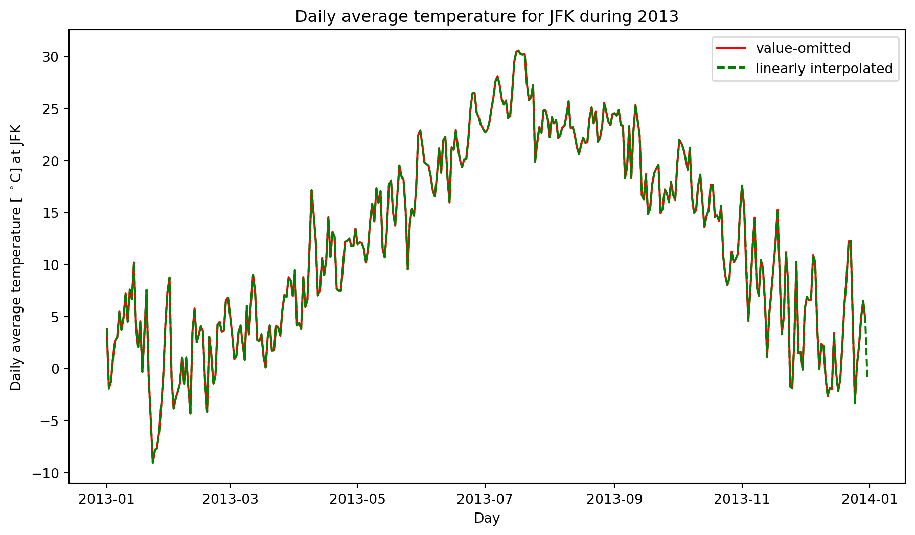
The only noticeable visual difference between the value-omitted and linearly interpolated daily average temperatures is on December 31st, where there is no data in the value-omitted, but data for the linearly interpolated.
Summary
This Jupyter Notebook demonstrates the use of pandas data frames to analyse time series meteorological data quantitatively using descriptive statistics and visually using line plots.
Possible extensions to the data analysis include: - Calculating the daily average wind speed at EWR and JFK for comparison with LGA. - Calculate a moving average and plot it with the daily average.