Supervised Learning

import pandas as pd
import numpy as np
import matplotlib.pyplot as plt
import seaborn as sns
import time

Introduction

Data pre-processing

Data

The dataset used in this part is the Bank Marketing from the UC Irvine Machine Learning Repository. The data is licensed under CC BY, allowing it to be freely used for this exercise.

The dataset contains data from direct marketing campaigns (phone calls) of a Portuguese banking institution. The data comprises 16 features and a labelled variable, “y”, which indicates if the client subscribed to a term deposit.

Load data

The data is loaded into a pandas dataframe from the downloaded CSV file. After loading the data, the first five rows of the dataframe are inspected using the head() function. The dataframe is then checked for any missing values. This dataset is clean with no missing values.

# Load the data file into a dataframe
bank_df = pd.read_csv("bank-full.csv", sep=";", comment="#")

# Inspect the head of the data
print(bank_df.head())

   age           job  marital  education default  balance housing loan  \
0   58    management  married   tertiary      no     2143     yes   no   
1   44    technician   single  secondary      no       29     yes   no   
2   33  entrepreneur  married  secondary      no        2     yes  yes   
3   47   blue-collar  married    unknown      no     1506     yes   no   
4   33       unknown   single    unknown      no        1      no   no   

   contact  day month  duration  campaign  pdays  previous poutcome   y  
0  unknown    5   may       261         1     -1         0  unknown  no  
1  unknown    5   may       151         1     -1         0  unknown  no  
2  unknown    5   may        76         1     -1         0  unknown  no  
3  unknown    5   may        92         1     -1         0  unknown  no  
4  unknown    5   may       198         1     -1         0  unknown  no  

Check for null values

# Check how many null values are in the data frame
print()
print("Feature Name           Number of missing entries")
print(bank_df.isnull().sum())

Feature Name           Number of missing entries
age          0
job          0
marital      0
education    0
default      0
balance      0
housing      0
loan         0
contact      0
day          0
month        0
duration     0
campaign     0
pdays        0
previous     0
poutcome     0
y            0
dtype: int64

Check for duplicate values

# Count duplicate rows
duplicate_count = bank_df.duplicated().sum()

print(f"Number of duplicate rows: {duplicate_count}")

Number of duplicate rows: 0

Drop irrelevant features

The dataset metadata states that the “duration” feature should only be included for benchmark purposes and should be discarded if the intention is to have a realistic predictive model.

bank_df.drop(["duration"], axis=1, inplace=True)

Feature encoding

The source of the dataset provides information relating to each variable, such as data type.

from sklearn.preprocessing import LabelEncoder
from sklearn.preprocessing import OneHotEncoder

Check datatypes

bank_df.info()

<class 'pandas.core.frame.DataFrame'>
RangeIndex: 45211 entries, 0 to 45210
Data columns (total 16 columns):
 #   Column     Non-Null Count  Dtype 
---  ------     --------------  ----- 
 0   age        45211 non-null  int64 
 1   job        45211 non-null  object
 2   marital    45211 non-null  object
 3   education  45211 non-null  object
 4   default    45211 non-null  object
 5   balance    45211 non-null  int64 
 6   housing    45211 non-null  object
 7   loan       45211 non-null  object
 8   contact    45211 non-null  object
 9   day        45211 non-null  int64 
 10  month      45211 non-null  object
 11  campaign   45211 non-null  int64 
 12  pdays      45211 non-null  int64 
 13  previous   45211 non-null  int64 
 14  poutcome   45211 non-null  object
 15  y          45211 non-null  object
dtypes: int64(6), object(10)
memory usage: 5.5+ MB

Check categorical features

# List of columns to inspect
selected_columns = ["job", "marital", "education", "default", "housing", "loan", "contact", "month", "poutcome"]

# Print unique values for each selected column
for column in selected_columns:
    unique_values = bank_df[column].unique()
    print(f"Unique values in column '{column}':")
    print(unique_values)
    print("-" *70)

Unique values in column 'job':
['management' 'technician' 'entrepreneur' 'blue-collar' 'unknown'
 'retired' 'admin.' 'services' 'self-employed' 'unemployed' 'housemaid'
 'student']
----------------------------------------------------------------------
Unique values in column 'marital':
['married' 'single' 'divorced']
----------------------------------------------------------------------
Unique values in column 'education':
['tertiary' 'secondary' 'unknown' 'primary']
----------------------------------------------------------------------
Unique values in column 'default':
['no' 'yes']
----------------------------------------------------------------------
Unique values in column 'housing':
['yes' 'no']
----------------------------------------------------------------------
Unique values in column 'loan':
['no' 'yes']
----------------------------------------------------------------------
Unique values in column 'contact':
['unknown' 'cellular' 'telephone']
----------------------------------------------------------------------
Unique values in column 'month':
['may' 'jun' 'jul' 'aug' 'oct' 'nov' 'dec' 'jan' 'feb' 'mar' 'apr' 'sep']
----------------------------------------------------------------------
Unique values in column 'poutcome':
['unknown' 'failure' 'other' 'success']
----------------------------------------------------------------------

Encoding nominal categorical features

The categorical features require encoding. One-hot encoding was applied to the nominal features: “job”, “marital”, “contact”, “month”, “default”, “housing”, “loan” and “poutcome”.

# Columns to encode
one_hot_cols = ["job", "marital", "default", "housing", "loan", "contact", "month", "poutcome"]

# OneHotEncoder setup
encoder = OneHotEncoder(sparse_output=False)
encoded = encoder.fit_transform(bank_df[one_hot_cols])

# Create DataFrame from encoded data
encoded_df = pd.DataFrame(encoded, columns=encoder.get_feature_names_out(one_hot_cols))

print(encoded_df.head())

#Copy the bank dataframe
en_bank_df= bank_df.copy()

# Drop original columns
en_bank_df = en_bank_df.drop(one_hot_cols, axis=1)

# Insert encoded columns before the last column
insert_position = en_bank_df.shape[1] - 1
for col in reversed(encoded_df.columns):
    en_bank_df.insert(insert_position, col, encoded_df[col])

   job_admin.  job_blue-collar  job_entrepreneur  job_housemaid  \
0         0.0              0.0               0.0            0.0   
1         0.0              0.0               0.0            0.0   
2         0.0              0.0               1.0            0.0   
3         0.0              1.0               0.0            0.0   
4         0.0              0.0               0.0            0.0   

   job_management  job_retired  job_self-employed  job_services  job_student  \
0             1.0          0.0                0.0           0.0          0.0   
1             0.0          0.0                0.0           0.0          0.0   
2             0.0          0.0                0.0           0.0          0.0   
3             0.0          0.0                0.0           0.0          0.0   
4             0.0          0.0                0.0           0.0          0.0   

   job_technician  ...  month_jun  month_mar  month_may  month_nov  month_oct  \
0             0.0  ...        0.0        0.0        1.0        0.0        0.0   
1             1.0  ...        0.0        0.0        1.0        0.0        0.0   
2             0.0  ...        0.0        0.0        1.0        0.0        0.0   
3             0.0  ...        0.0        0.0        1.0        0.0        0.0   
4             0.0  ...        0.0        0.0        1.0        0.0        0.0   

   month_sep  poutcome_failure  poutcome_other  poutcome_success  \
0        0.0               0.0             0.0               0.0   
1        0.0               0.0             0.0               0.0   
2        0.0               0.0             0.0               0.0   
3        0.0               0.0             0.0               0.0   
4        0.0               0.0             0.0               0.0   

   poutcome_unknown  
0               1.0  
1               1.0  
2               1.0  
3               1.0  
4               1.0  

[5 rows x 40 columns]

Encoding ordinal categorical features

Ordinal encoding was applied to the ordinal feature “education”, as its ordering is important.

# Ordinal encoding
# Education ordinal mapping
education_mapping = {
    "unknown": 0,
    "primary": 1,
    "secondary": 2,
    "tertiary": 3
}

# Apply the mapping
en_bank_df["education"] = en_bank_df["education"].map(education_mapping)

# Display the updated dataframe with encoded columns.
print(en_bank_df[["education"]].head())

   education
0          3
1          2
2          2
3          0
4          0

Target encoding

# Create label encoder
le = LabelEncoder()

en_bank_df = en_bank_df.rename(columns={"y": "target"})

en_bank_df["target"] = le.fit_transform(en_bank_df["target"])
en_bank_df.head(5)

	age	education	balance	day	campaign	pdays	previous	job_admin.	job_blue-collar	job_entrepreneur	...	month_mar	month_may	month_nov	month_oct	month_sep	poutcome_failure	poutcome_other	poutcome_success	poutcome_unknown	target
0	58	3	2143	5	1	-1	0	0.0	0.0	0.0	...	0.0	1.0	0.0	0.0	0.0	0.0	0.0	0.0	1.0	0
1	44	2	29	5	1	-1	0	0.0	0.0	0.0	...	0.0	1.0	0.0	0.0	0.0	0.0	0.0	0.0	1.0	0
2	33	2	2	5	1	-1	0	0.0	0.0	1.0	...	0.0	1.0	0.0	0.0	0.0	0.0	0.0	0.0	1.0	0
3	47	0	1506	5	1	-1	0	0.0	1.0	0.0	...	0.0	1.0	0.0	0.0	0.0	0.0	0.0	0.0	1.0	0
4	33	0	1	5	1	-1	0	0.0	0.0	0.0	...	0.0	1.0	0.0	0.0	0.0	0.0	0.0	0.0	1.0	0

5 rows × 48 columns

Dataset balance

Here I inspect the blance of the classes in the full dataset. The figure below shows there is many more no’s (0) and yes’s (1).

# Count distribution of 0s and 1s
target_counts = en_bank_df["target"].value_counts()

# Plot the distribution
plt.figure(figsize=(6, 4))
target_counts.plot(kind="bar", color=["skyblue", "orange"])
plt.title("Distribution of Target Variable")
plt.xlabel("Target Class")
plt.ylabel("Count")
plt.xticks(ticks=[0, 1], labels=["0 (no)", "1 (yes)"], rotation=0)
plt.tight_layout()
plt.show()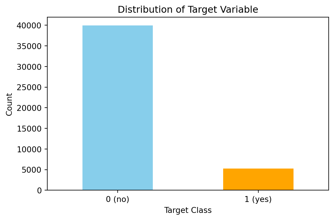

Handling dataset imbalance

It has been observed that the dataset is imbalanced with approximately 11% of the data in the “yes” class and the remaining in the “no” class. There are several ways to handle imbalanced datasets, such as under-sampling the majority class, oversampling the minority class, SMOTE, and cost-sensitive learning, where the weights of each class are adjusted to adjust the cost function. I tested both SMOTE and found that the increased training set size caused problems with overfitting in the K-NN section. Therefore, here I have opted to use cost-sensitive learning.

Train test split

Stratified sampling has been used to ensure the class proporations remaing the same in the test and train sets.

from sklearn.model_selection import StratifiedShuffleSplit
from sklearn.preprocessing import StandardScaler

# Split the data
# Stratified sampling to help maintain similar distributions between the text and train sets
stratSplit = StratifiedShuffleSplit(n_splits=1, test_size=0.2, random_state=8)
for train_index, test_index in stratSplit.split(en_bank_df.iloc[:, :-1], en_bank_df["target"]):
    X_train = en_bank_df.iloc[:, :-1].iloc[train_index]
    X_test = en_bank_df.iloc[:, :-1].iloc[test_index]
    y_train = en_bank_df["target"].iloc[train_index]
    y_test = en_bank_df["target"].iloc[test_index]

# Fit scaler on training data
scaler = StandardScaler()
X_train_scald = scaler.fit_transform(X_train)

# Transform test data using the same scaler
X_test_scald = scaler.transform(X_test)

# check class distribution in test set
test_counts = y_test.value_counts()

# check null accuracy score
null_accuracy = (test_counts[0]/(test_counts[0] + test_counts[1]))

print(f"Null accuracy score: {null_accuracy:.4f}")

Null accuracy score: 0.8830

First logistic regression (no regularisation)

Here, a logistic regression model is fitted without any regularisation. The logistic regression model in scikit learn has several hyperparameters. Those specific to the non-regularised version are:

• Solver: The type of solver used.
• Maximum Iterations: Controls how long the solver runs.
• Tolerance: Determines the stopping criteria for the optimisation.
• Class Weight: Useful for imbalanced datasets.

Since I will be creating regularised logistic models for this data later, I decided to remove the solver from the hyperparameter tuning. There is only one solver (“saga”) that handles no regularisation and the L1 and L2 regularisation, and I want to use the same solver for each model.

Hyperparameter tuning

For the model evaluation, I have used the F1 score. F1 is the harmonic mean of precision and recall. The main objective of this modelling work is to predict whether a customer will subscribe to a term deposit. Therefore, I aim to strike a balance between the recall (don’t want to miss potential conversions) and the precision (don’t want to waste effort on uninterested people).

The scikit learn GridSearchCV is used to execute the parameter tuning. It runs through all combinations of the parameters and uses cross-validation to assess the performance of the model. The results showed that the maximum number of iterations and convergence tolerance were not significant compared to the class weights.

from sklearn.linear_model import LogisticRegression
from sklearn.model_selection import GridSearchCV
from sklearn.pipeline import Pipeline

# Define pipeline (logistic regression)
pipeline = Pipeline([
    ("logreg", LogisticRegression(penalty=None, solver="saga", random_state=8))
])

param_grid = {
    "logreg__class_weight": [
        None,
        'balanced',
        {0: 1, 1: 2.5},  
        {0: 1, 1: 5},
        {0: 1, 1: 10}
    ],
    "logreg__max_iter": [100, 500, 1000],
    "logreg__tol": [1e-5, 1e-4, 1e-3],
}

# Set up GridSearchCV
# GridSearchCV uses stratified sampling internally, so need to do anything special here.
# Only interested in minorty class so don't weight score
grid_search = GridSearchCV(pipeline, param_grid, cv=5, scoring="f1", n_jobs=-1, return_train_score=True)

# Fit the model
grid_search.fit(X_train_scald, y_train)

# Convert results to DataFrame
results_df = pd.DataFrame(grid_search.cv_results_)

# Create a readable label for each parameter combination
results_df["param_combo"] = results_df.apply(
    lambda row: f"{row['param_logreg__max_iter']}, tol={row['param_logreg__tol']}, weight={row['param_logreg__class_weight']}",
    axis=1
)

# Sort by mean test score
results_df = results_df.sort_values(by="mean_test_score", ascending=False)

# Plot performance of each combination in grid search
plt.figure(figsize=(12, 12))
plt.barh(results_df["param_combo"], results_df["mean_test_score"], color="skyblue")
plt.xlabel("Mean Score")
plt.title("Grid Search Results for Logistic Regression (No Regularisation)")
plt.gca().invert_yaxis()
plt.tight_layout()
plt.grid(True)
plt.show()

# Best parameters and score
print("Best Parameters:", grid_search.best_params_)
print(f"Best Score: {grid_search.best_score_:.4f}")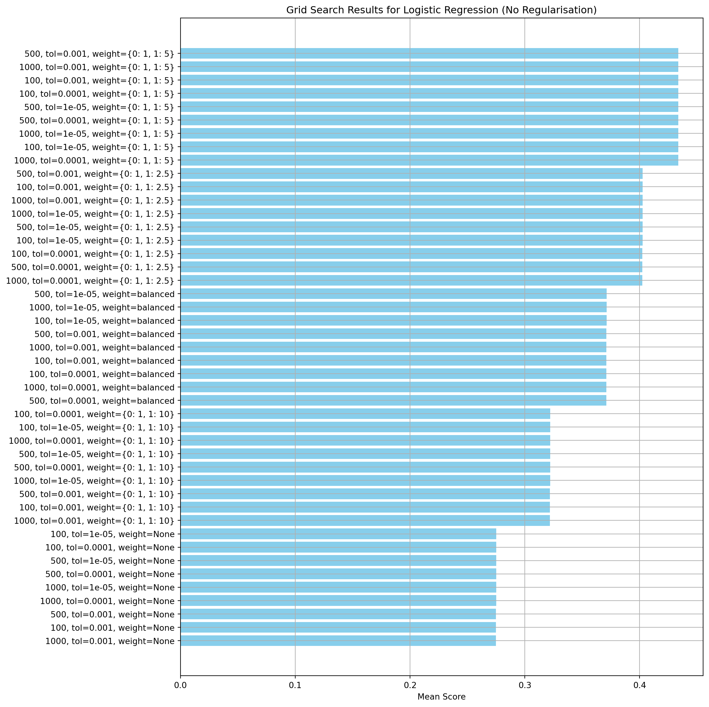

Best Parameters: {'logreg__class_weight': {0: 1, 1: 5}, 'logreg__max_iter': 100, 'logreg__tol': 0.001}
Best Score: 0.4336

Create a model with the best parameters and run cross-validation

Here, I’m using cross-validation to check the model’s ability to generalise. Looking for divergence between the training and validation scores. The results show the model is stable and not over-fitted.

from sklearn.model_selection import cross_validate

def performCV(model, X_train, y_train):
    """
    Function to perform cross-validation for a given model and training data.

    :param model: The model to validate.
    :param X_train: Training data.
    :param y_train: TRaining labels.
    :returns: Dictionary of results from the cross-validation.
    """
    results = cross_validate(model, X=X_train, y=y_train,
                    scoring=["f1", "precision", "recall", "accuracy", "roc_auc"],                         
                    cv=5, verbose=True, return_train_score=True,
                    return_estimator=True)
    return results


def visualiseResults(results):
    """
    Function to plot different scoring metrics from a cross-validsation
    study.

    :param results: Dictionary containing the cross-validation results.
    :returns: None.
    """
    cvData = {"val_f1":results["test_f1"],
            "train_f1":results["train_f1"],
            "val_precision":results["test_precision"],
            "train_precision":results["train_precision"],
            "val_recall":results["test_recall"],
            "train_recall":results["train_recall"],
            "val_acc":results["test_accuracy"],
            "train_acc":results["train_accuracy"],
            "val_roc_auc":results["test_roc_auc"],
            "train_roc_auc":results["train_roc_auc"]}

    cv_df = pd.DataFrame(cvData)
    fig = plt.figure(figsize=(8,6))
    ax = fig.add_subplot()
    plt.plot(cv_df.index, cv_df["train_acc"], label="train_acc", color="r")
    plt.plot(cv_df.index, cv_df["val_acc"], label="val_acc", c="r", ls="--")
    plt.plot(cv_df.index, cv_df["train_f1"], label="train_f1", c="b")
    plt.plot(cv_df.index, cv_df["val_f1"], label="val_f1", c="b", ls="--")
    plt.plot(cv_df.index, cv_df["train_recall"], label="train_recall", c="g")
    plt.plot(cv_df.index, cv_df["val_recall"], label="val_recall", c="g", ls="--")
    plt.plot(cv_df.index, cv_df["train_precision"], label="train_precision", c="purple")
    plt.plot(cv_df.index, cv_df["val_precision"], label="val_precision", c="purple", ls="--")
    plt.plot(cv_df.index, cv_df["train_roc_auc"], label="train_roc_auc", c="magenta")
    plt.plot(cv_df.index, cv_df["val_roc_auc"], label="val_roc_auc", c="magenta", ls="--")
    plt.legend()
    plt.ylabel("Score")
    plt.title("Model performance based on multiple scoring metrics")
    plt.xticks(range(len(results["fit_time"])),["run "+str(i+1) for i in range(len(results["fit_time"]))])
    plt.show()

# Create the model using the best parameters found in the hyperparameter tuning step
log_reg_nr = LogisticRegression(penalty=None, solver="saga", max_iter=400, tol=0.001, class_weight={0: 1, 1: 5}, random_state=8)

# Run cross-validation
cv_results = performCV(log_reg_nr, X_train_scald, y_train)
visualiseResults(cv_results)

[Parallel(n_jobs=1)]: Done   5 out of   5 | elapsed:    1.1s finished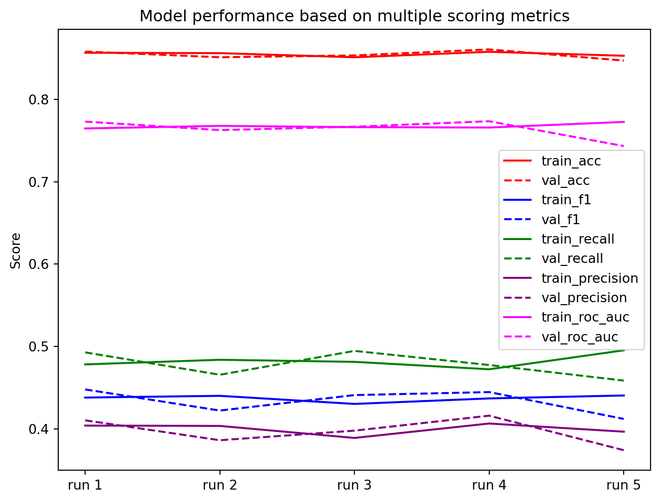

Evaluate model performance

Here, I evaluate the model’s performance by calculating the precision, recall, F1 score and the ROC_AUC score. The confusion matrix is also plotted. The recall and precision are very good for the majority class, as expected, due to the class imbalance. The minority class shows the precision is approximately 42% and the recall is approximately 50%.

from sklearn.metrics import classification_report
from sklearn.metrics import confusion_matrix, ConfusionMatrixDisplay
from sklearn.metrics import roc_auc_score

log_reg_nr.fit(X_train_scald, y_train)
y_pred = log_reg_nr.predict(X_test_scald)

print(classification_report(y_test, y_pred, target_names=["no", "yes"], digits=4))

# Predict probabilities
y_probs = log_reg_nr.predict_proba(X_test_scald)[:, 1]  # Probabilities for class 1

# Compute ROC AUC
roc_auc = roc_auc_score(y_test, y_probs)
print(f"ROC AUC Score: {roc_auc:.4f}")

cm_nr = confusion_matrix(y_test, y_pred, labels=[0,1])

              precision    recall  f1-score   support

          no     0.9319    0.9088    0.9202      7985
         yes     0.4204    0.4991    0.4564      1058

    accuracy                         0.8609      9043
   macro avg     0.6762    0.7039    0.6883      9043
weighted avg     0.8721    0.8609    0.8660      9043

ROC AUC Score: 0.7735

Second and Third logistic regression models

In this second two additional logistic regission models are created with differing regularisation to invesitigate if regularisation affects the performance of the model for this application.

LASSO regularisation (L1)

This section creates a regularisation model using the L1 norm. Firstly, I run a grid search to find the value of C and the class weights that give the highest F1 score. Other parameters, such as convergence tolerance, maximum solver iterations and class weights have been set to the same values used for the non-regularised model. Like the non-regularised model, the class weights have the most effect on the model performance. The value of the regularisation strength (C) has little effect once the optimal class weights are selected.

# LASSO - L1
# Define pipeline
lasso_pipeline = Pipeline([
    ("lasso", LogisticRegression(penalty="l1", solver="saga", random_state=8,
                                 tol=1e-3, max_iter=400, class_weight=None))
])

# Define parameter grid
lasso_params = {
    "lasso__C": [0.0001, 0.001, 0.01, 0.1, 1.0, 10.0, 100.0],
     "lasso__class_weight": [
        None,
        'balanced',
        {0: 1, 1: 2.5},  
        {0: 1, 1: 5},
        {0: 1, 1: 10}
    ]
}

# Set up GridSearchCV
lasso_grid_search = GridSearchCV(lasso_pipeline, lasso_params, cv=5, scoring="f1", n_jobs=-1, return_train_score=True)

# Fit the model
lasso_grid_search.fit(X_train_scald, y_train)

# Convert results to DataFrame
lasso_results_df = pd.DataFrame(lasso_grid_search.cv_results_)

# Create a readable label for each parameter combination
lasso_results_df["param_combo"] = lasso_results_df.apply(
    lambda row: f"{row['param_lasso__C']},  weight={row['param_lasso__class_weight']}",
    axis=1
)

# Sort by mean test score
lasso_results_df = lasso_results_df.sort_values(by="mean_test_score", ascending=False)

# Plot performance of each combination in grid search
plt.figure(figsize=(12, 8))
plt.barh(lasso_results_df["param_combo"], lasso_results_df["mean_test_score"], color="skyblue")
plt.xlabel("Mean Score")
plt.title("Grid Search Results for Logistic Regression (LASSO Regularisation)")
plt.gca().invert_yaxis()
plt.tight_layout()
plt.grid(True)
plt.show()

# Best parameters and score
print("Best Parameters:", lasso_grid_search.best_params_)
print(f"Best Score: {lasso_grid_search.best_score_:.4f}")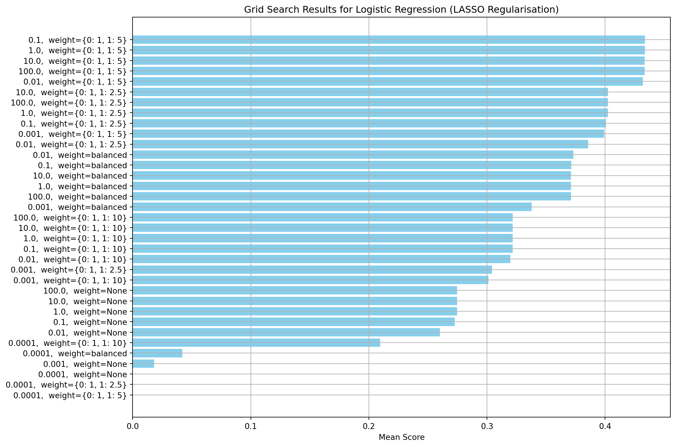

Best Parameters: {'lasso__C': 0.1, 'lasso__class_weight': {0: 1, 1: 5}}
Best Score: 0.4337

log_reg_l1 = LogisticRegression(penalty="l1", solver="saga", max_iter=400, tol=0.001, class_weight= {0: 1, 1: 5}, C=0.1)

Ridge regularisation (L2)

This section creates a regularisation model using the L2 norm. Firstly, I run a grid to find the values of C and class weights that give the highest F1 score. Other parameters, such as convergence tolerance, maximum solver iterations and class weights have been set to the same values used for the non-regularised model. Similar to the other two models, the class weights are the most important parameter. The regularisation strength has no effect for values about 0.1

# Ridge - L2
# Define pipeline
ridge_pipeline = Pipeline([
    ("ridge", LogisticRegression(penalty="l2", solver="saga", random_state=8,
                                 tol=1e-5, max_iter=100, class_weight=None))
])

# Define parameter grid
ridge_params = {
    "ridge__C": [0.0001, 0.001, 0.01, 0.1, 1.0, 10.0],
     "ridge__class_weight": [
        None,
        'balanced',
        {0: 1, 1: 2.5},  
        {0: 1, 1: 5},
        {0: 1, 1: 10}
    ]
}

# Set up GridSearchCV
ridge_grid_search = GridSearchCV(ridge_pipeline, ridge_params, cv=5, scoring="f1", n_jobs=-1, return_train_score=True)

# Fit the model
ridge_grid_search.fit(X_train_scald, y_train)

# Convert results to DataFrame
ridge_results_df = pd.DataFrame(ridge_grid_search.cv_results_)

# Create a readable label for each parameter combination
ridge_results_df["param_combo"] = ridge_results_df.apply(
    lambda row: f"{row['param_ridge__C']},  weight={row['param_ridge__class_weight']}",
    axis=1
)

# Sort by mean test score
ridge_results_df = ridge_results_df.sort_values(by="mean_test_score", ascending=False)

# Plot performance of each combination in grid search
plt.figure(figsize=(12, 8))
plt.barh(ridge_results_df["param_combo"], ridge_results_df["mean_test_score"], color="skyblue")
plt.xlabel("Mean Score")
plt.title("Grid Search Results for Logistic Regression (Ridge Regularisation)")
plt.gca().invert_yaxis()
plt.tight_layout()
plt.grid(True)
plt.show()

# Best parameters and score
print("Best Parameters:", ridge_grid_search.best_params_)
print(f"Best Score: {ridge_grid_search.best_score_:.4f}")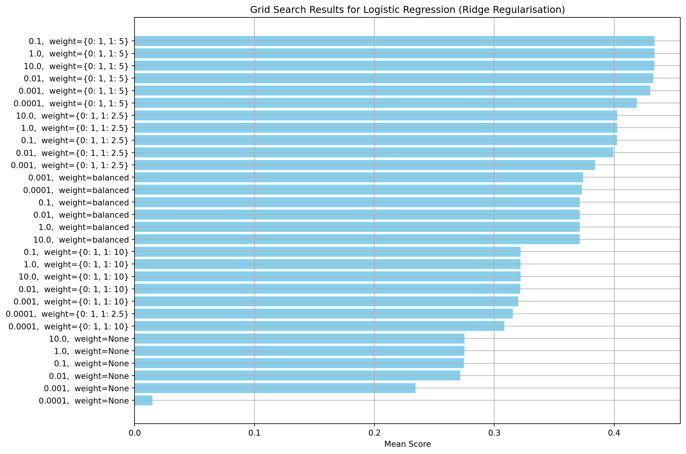

Best Parameters: {'ridge__C': 0.1, 'ridge__class_weight': {0: 1, 1: 5}}
Best Score: 0.4337

log_reg_l2 = LogisticRegression(penalty="l2", solver="saga", random_state=8,
                                 max_iter=400, tol=1e-3, class_weight= {0: 1, 1: 5}, C=0.1)

Comparsion of 1st, 2nd and 3rd models

In this section, I compare the performance of the three logistic models.

The performance metrics are virtually identical across all three models (differences in the third decimal place), which confirms that regularisation isn’t providing meaningful benefit here. This suggests the first model is already well-calibrated without regularisation. Since regularisation isn’t having any effect, the models are not overfitting. The logistic regression coefficients for each model have also been printed and compared.

Comparison Summary

Model	Recall (yes)	Precision (yes)	F1 Score (yes)	ROC_AUC score (yes)
No Regularization	0.4991	0.4564	0.4204	0.7735
L1 Regularization	0.4981	0.4565	0.4213	0.7738
L2 Regularization	0.4991	0.4565	0.4204	0.7736

The coefficients are remarkably similar across all three models (no regularisation, L1, and L2), which suggests:

• Model Stability - The fact that regularisation barely changes the coefficients suggests the first model wasn’t significantly overfitting. If there were overfitting, I’d expect to see much larger differences when regularisation is applied.
• Feature importance is consistent between the non-regularised and L2 models. The first two largest coefficients are consistent across all models:
  • poutcome_sucess: ~0.36 (strongest positive predictor)
  • contact_unknown: ~-0.33 (strongest negative predictor)
• L1 vs L2 Differences - L1 regularisation typically drives some coefficients to exactly zero (feature selection), while L2 shrinks them toward zero. The L1 model is driving four coefficients to zero, which reinforces that most features are contributing meaningful information.

import matplotlib.pyplot as plt
import seaborn as sns
import numpy as np

# Define confusion matrices based on the provided metrics

# L1 regularization
log_reg_l1.fit(X_train_scald, y_train)
y_pred_l1 = log_reg_l1.predict(X_test_scald)
cm_l1 = confusion_matrix(y_test, y_pred_l1, labels=[0,1])
print("L1 regularisation results:")
print(classification_report(y_test, y_pred_l1, target_names=["no", "yes"], digits=4))
y_probs_l1 = log_reg_l1.predict_proba(X_test_scald)[:, 1]  # Probabilities for class 1
roc_auc_l1 = roc_auc_score(y_test, y_probs_l1)
print(f"ROC AUC Score: {roc_auc_l1:.4f}")

# L2 regularization
start_fit = time.perf_counter()
log_reg_l2.fit(X_train_scald, y_train)
end_fit = time.perf_counter()

start_pred = time.perf_counter()
y_pred_l2 = log_reg_l2.predict(X_test_scald)
end_pred =time.perf_counter()

cm_l2 = confusion_matrix(y_test, y_pred_l2, labels=[0,1])
print("L2 regularisation results:")
print(classification_report(y_test, y_pred_l2, target_names=["no", "yes"], digits=4))
y_probs_l2 = log_reg_l2.predict_proba(X_test_scald)[:, 1]  # Probabilities for class 1
roc_auc_l2 = roc_auc_score(y_test, y_probs_l2)
print(f"ROC AUC Score: {roc_auc_l2:.4f}")

# Report timings
log_reg_l2_fit_time = end_fit - start_fit
log_reg_l2_pred_time = end_pred - start_pred

print(f"Log Regression (L2) fitting time: {log_reg_l2_fit_time:.4f} seconds")
print(f"Log Regression (L2) prediction time: {log_reg_l2_pred_time:.4e} seconds")

# Plotting function
def plot_confusion_matrix(cm, title, ax):
    sns.heatmap(cm, annot=True, fmt='d', cmap='Blues', cbar=False, ax=ax)
    ax.set_title(title)
    ax.set_xlabel('Predicted')
    ax.set_ylabel('Actual')
    ax.set_xticklabels(['no', 'yes'])
    ax.set_yticklabels(['no', 'yes'])

# Create subplots
fig, axes = plt.subplots(1, 3, figsize=(18, 5))

plot_confusion_matrix(cm_nr, 'No Regularization', axes[0])
plot_confusion_matrix(cm_l1, 'L1 Regularization', axes[1])
plot_confusion_matrix(cm_l2, 'L2 Regularization', axes[2])

plt.tight_layout()
plt.show()

L1 regularisation results:
              precision    recall  f1-score   support

          no     0.9319    0.9093    0.9205      7985
         yes     0.4213    0.4981    0.4565      1058

    accuracy                         0.8612      9043
   macro avg     0.6766    0.7037    0.6885      9043
weighted avg     0.8721    0.8612    0.8662      9043

ROC AUC Score: 0.7738
L2 regularisation results:
              precision    recall  f1-score   support

          no     0.9319    0.9088    0.9202      7985
         yes     0.4204    0.4991    0.4564      1058

    accuracy                         0.8609      9043
   macro avg     0.6762    0.7039    0.6883      9043
weighted avg     0.8721    0.8609    0.8660      9043

ROC AUC Score: 0.7736
Log Regression (L2) fitting time: 0.5195 seconds
Log Regression (L2) prediction time: 1.3113e-03 seconds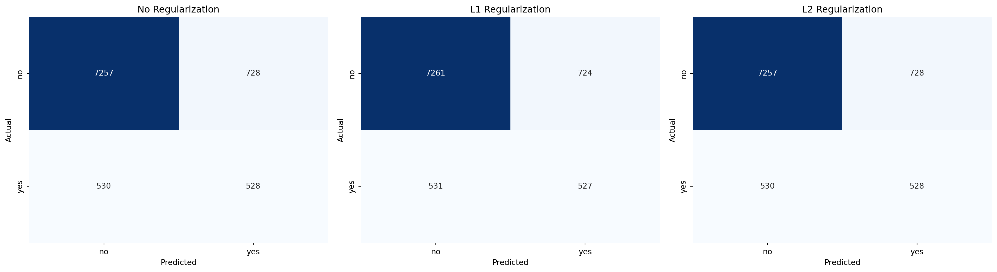

feature_names = X_train.columns
coefs_nr = log_reg_nr.coef_.flatten()
coefs_l1 = log_reg_l1.coef_.flatten()
coefs_l2 = log_reg_l2.coef_.flatten()

logistic_nr = pd.DataFrame({'feature_name': feature_names, 'coefficients': coefs_nr})
logistic_l1 = pd.DataFrame({'feature_name': feature_names, 'coefficients': coefs_l1})
logistic_l2 = pd.DataFrame({'feature_name': feature_names, 'coefficients': coefs_l2})
results = [logistic_nr, logistic_l1, logistic_l2]

fig, axes = plt.subplots(3, 1, figsize=(8, 21))
subplot_titles=["No regularisation", "L1 regularisation", "L2 regularisation"]

for i, ax in enumerate(axes):
    # Sort the features by the absolute value of their coefficient
    results[i]["abs_value"] = results[i]["coefficients"].apply(lambda x: abs(x))
    #results[i]["colors"] = results[i]["coefficients"].apply(lambda x: "green" if x > 0 else "red")
    results[i] = results[i].sort_values("abs_value", ascending=False)
    
    sns.barplot(x="feature_name", y="coefficients", data=results[i].head(20),ax=ax)

    # Colour bars based on coefficient sign
    for bar, coeff in zip(ax.patches, results[i]['coefficients']):
        bar.set_color('green' if coeff >= 0 else 'red')

    axes[i].set_xlabel("Feature Name", fontsize=12)
    
    tick_positions = range(20)
    ax.set_xticks(tick_positions)
    ax.set_xticklabels(results[i]["feature_name"].head(20), rotation=45, ha='right')
    axes[i].set_ylabel("Coef", fontsize=12)    
    axes[i].tick_params(axis='x', labelrotation=45)
    ax.set_title(subplot_titles[i])

# Rotate x-axis labels for better readability
plt.xticks(rotation=45, ha='right')
fig.suptitle("Top 20 Features Logistic Regression", fontsize=14)
plt.tight_layout(rect=[0, 0, 1, 0.99])
plt.show()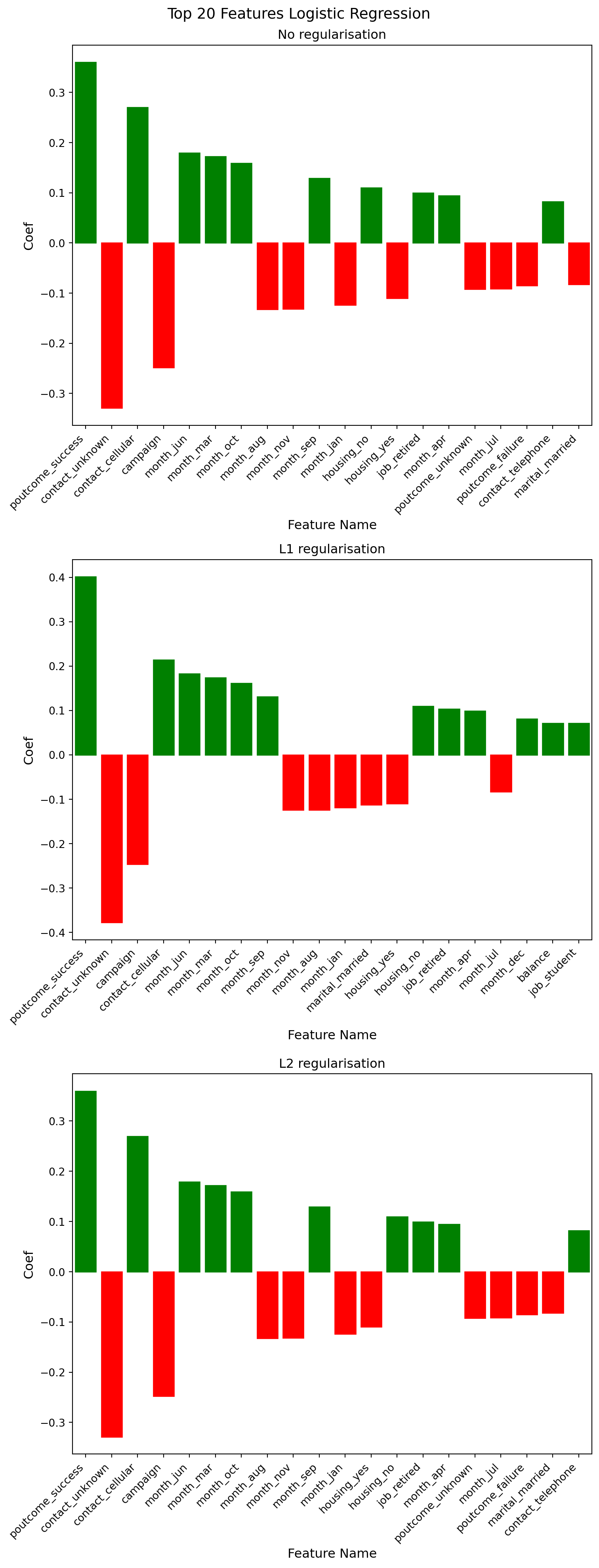

# Compare feature selection between L1 and L2
print(f"L1 non-zero features: {np.sum(log_reg_l1.coef_[0] != 0)}")
print(f"L2 non-zero features: {np.sum(log_reg_l2.coef_[0] != 0)}")
print(f"Total features: {len(log_reg_l1.coef_[0])}")

L1 non-zero features: 43
L2 non-zero features: 47
Total features: 47

print("Features removed from L1 model:")
logistic_l1[logistic_l1["coefficients"] == 0]

Features removed from L1 model:

	feature_name	coefficients	abs_value
16	job_technician	0.0	0.0
19	marital_divorced	0.0	0.0
39	month_may	0.0	0.0
46	poutcome_unknown	0.0	0.0

from sklearn.metrics import precision_recall_curve
from sklearn.metrics import roc_curve

yRawScores_nr = log_reg_nr.decision_function(X_train_scald)
yRawScores_l1 = log_reg_l1.decision_function(X_train_scald)
yRawScores_l2 = log_reg_l2.decision_function(X_train_scald)

fpr_nr, tpr_nr, thresholds_nr = roc_curve(y_train, yRawScores_nr)
fpr_l1, tpr_l1, thresholds_l1 = roc_curve(y_train, yRawScores_l1)
fpr_l2, tpr_l2, thresholds_l2 = roc_curve(y_train, yRawScores_l2)

plt.figure(figsize=(8,8))
plt.plot(fpr_nr,tpr_nr, label="no regularisation")
plt.plot(fpr_l1,tpr_l1, label="L1 regularisation")
plt.plot(fpr_l2,tpr_l2, label="L2 regularisation")
plt.xlabel("FPR",fontsize=15)
plt.ylabel("Recall (TPR)",fontsize=15)
plt.title("ROC",fontsize=20)

randomAssignment = np.random.normal(size=len(y_train))
fprRand, tprRand, thresholdsRand = roc_curve(y_train, randomAssignment)
plt.plot(fprRand, tprRand, ls="--", label="random classifier")
plt.legend()
plt.show()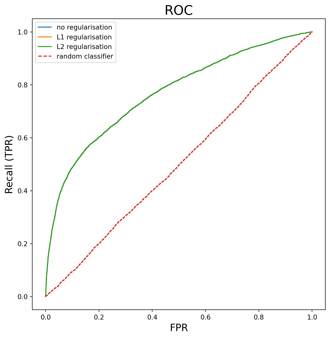

K-Nearest-Neighbour (KNN)

In this section, I fit a KNN model to the data. First, I use a grid search to find the optimal settings for K, the number of neighbours and the weights. The scoring of the model uses the F1 score to be consistent with the Logistic regression model produced earlier in this work.

from sklearn.neighbors import KNeighborsClassifier
from sklearn.model_selection import GridSearchCV
from sklearn.pipeline import Pipeline
import numpy as np

# Create pipeline
pipeline = Pipeline([
    ('knn', KNeighborsClassifier())
])

# Define K range to search
n_samples = len(X_train_scald)
sqrt_n = int(np.sqrt(n_samples))

# Test around this value
k_range = list(range(1, min(sqrt_n * 2, 50))) 

param_grid = {
    'knn__n_neighbors': k_range,
    'knn__weights': ['uniform', 'distance'],
}

# Grid search with CV
knn_grid_search = GridSearchCV(
    pipeline, 
    param_grid, 
    cv=5,
    scoring='f1',
    n_jobs=-1
)

knn_grid_search.fit(X_train_scald, y_train)
print(f"Best K: {knn_grid_search.best_params_}")
print(f"Best Score: {knn_grid_search.best_score_:.4f}")

Best K: {'knn__n_neighbors': 11, 'knn__weights': 'distance'}
Best Score: 0.3377

import matplotlib.pyplot as plt
from sklearn.model_selection import cross_val_score

# Extract results
k_scores = []
for k in k_range:
    knn = KNeighborsClassifier(n_neighbors=k, weights="distance")
    scores = cross_val_score(knn, X_train_scald, y_train, cv=5, scoring="f1")
    k_scores.append(scores.mean())

plt.plot(k_range, k_scores)
plt.xlabel("K")
plt.ylabel("F1 Score")
plt.title("KNN Performance vs K")
plt.show()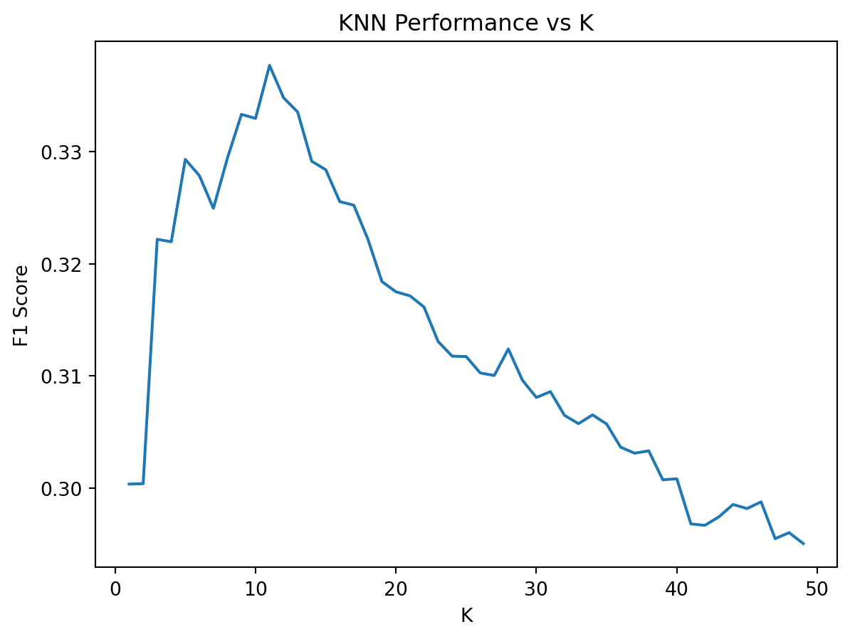

knn_model = KNeighborsClassifier(n_neighbors=11, weights="distance")

start_fit = time.perf_counter()
knn_model.fit(X_train_scald, y_train)
end_fit = time.perf_counter()

start_pred = time.perf_counter()
y_pred_knn = knn_model.predict(X_test_scald)
end_pred = time.perf_counter()

print(classification_report(y_test, y_pred_knn, target_names=["no", "yes"], digits=4))
y_probs_knn = knn_model.predict_proba(X_test_scald)[:, 1]  # Probabilities for class 1
roc_auc_knn = roc_auc_score(y_test, y_probs_knn)
print(f"ROC AUC Score: {roc_auc_knn:.4f}")
# Report timings
knn_fit_time = end_fit - start_fit
knn_pred_time = end_pred - start_pred

print(f"KNN fitting time: {knn_fit_time:.4f} seconds")
print(f"KNN prediction time: {knn_pred_time:.4f} seconds")

              precision    recall  f1-score   support

          no     0.9077    0.9752    0.9402      7985
         yes     0.5733    0.2514    0.3495      1058

    accuracy                         0.8905      9043
   macro avg     0.7405    0.6133    0.6449      9043
weighted avg     0.8686    0.8905    0.8711      9043

ROC AUC Score: 0.7391
KNN fitting time: 0.0062 seconds
KNN prediction time: 0.6241 seconds

Comparsion between Logistic regression and KNN models

# Calculate confusion matrix for KNN
knn_cm = confusion_matrix(y_test, y_pred_knn, labels=[0,1])

# Plot confusion matrices
fig, axes = plt.subplots(1, 2, figsize=(12, 5))

labels = ['no', 'yes']

# KNN Confusion Matrix
sns.heatmap(knn_cm, annot=True, fmt='d', cmap='Blues', ax=axes[0])
axes[0].set_title('KNN Confusion Matrix')
axes[0].set_xlabel('Predicted')
axes[0].set_ylabel('Actual')
axes[0].set_xticklabels(labels)
axes[0].set_yticklabels(labels)

# Logistic Regression Confusion Matrix
sns.heatmap(cm_l2, annot=True, fmt='d', cmap='Greens', ax=axes[1])
axes[1].set_title('Logistic Regression (L2) Confusion Matrix')
axes[1].set_xlabel('Predicted')
axes[1].set_ylabel('Actual')
axes[1].set_xticklabels(labels)
axes[1].set_yticklabels(labels)

plt.tight_layout()
plt.show()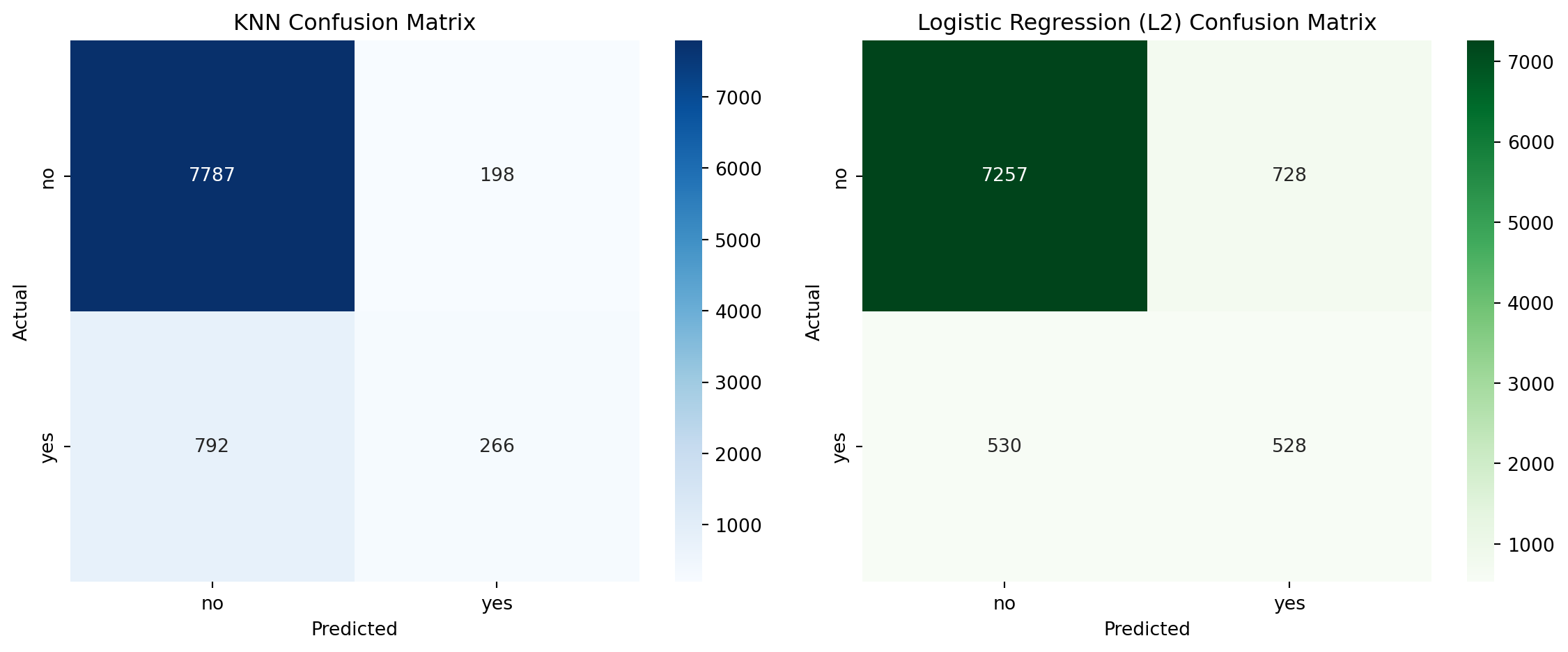

Performance Comparison: KNN vs Logistic Regression

Minority class (“yes”) metrics

Metric	Logistic Regression (L2)	KNN
Precision	0.4204	0.5733
Recall	0.4991	0.2514
F1 Score	0.4564	0.3495

Observation: KNN has low recall for the “yes” class, meaning it misses most of the actual positive cases. This is critical in marketing, where identifying potential responders is key. It does have higher precision, which means less time would be wasted on potential “no” responders.

Overall metrics

Metric	Logistic Regression (L2)	KNN
Accuracy	0.8609	0.8905
Macro F1	0.6883	0.6449
Weighted F1	0.8663	0.8711
ROC_AUC	0.7736	0.7391

Observation: KNN performs well on the majority class (“no”) but poorly on the minority class (“yes”), dragging down macro and weighted averages.

Training time

Model	Training Time (s)	Prediction Time (s)
Logistic Regression (L2)	0.1785	1.154200e-03
KNN	0.01	0.3590

KNN is faster at training because it simply stores the numbers and doesn’t do any calculations. However, it is much slower at prediction, because it does the calculations at that point. Based on the sum of training and prediction, Logistic Regression is faster overall.

Number of trainable parameters

Model	Trainable Parameters
Logistic Regression	Weights for each feature (plus bias). For binary classification with n features, it learns n + 1 parameters.
KNN	Stores the training data and makes decisions at prediction time, and has no trainable parameters.

Logistic Regression is more compact and interpretable.

Conclusion

For this application, KNN was worse than Logistic Regression because:

• KNN was worse at identifying “yes” cases, which is crucial in marketing.
• KNN had a faster training time but slower prediction time. This was noticeable when testing SMOTE (not shown in this notebook).