Basic Deep Learning

import tensorflow as tf
from tensorflow import keras
import matplotlib.pyplot as plt
import numpy as np
from tensorflow.keras.layers import Dense
from tensorflow.keras.models import Sequential

Load dataset

The datset is the MINIST Digist dataset obtained from the Keras package.

# Load the MNIST Dataset
(x_train, y_train), (x_test, y_test) = keras.datasets.mnist.load_data()

Training and test set sizes

# Print training set size
n_samples_train = x_train.shape[0]
print(f"Training set size: {n_samples_train} images")

n_samples_test = x_test.shape[0]
# Print test set size
print(f"Test set size: {n_samples_test} images")

Training set size: 60000 images
Test set size: 10000 images

Data Preprocessing

# Reshape the data to flatten the images
x_train_flat = x_train.reshape((n_samples_train, -1))
x_test_flat = x_test.reshape((n_samples_test, -1))

# Normalise pixel values to be between 0 and 1
x_train_flat = x_train_flat / 255.0
x_test_flat = x_test_flat / 255.0

# One-hot encode the labels
y_train = keras.utils.to_categorical(y_train, num_classes=10)
y_test = keras.utils.to_categorical(y_test, num_classes=10)

One hidden layer MLP model

# Develop a one hidden layer MLP model
model_one_layer = Sequential([
    Dense(100, activation="relu"), # Hidden layer
    Dense(10, activation="softmax") # Output layer
])

# Make the model
model_one_layer.compile(
    optimizer="adam",
    loss="categorical_crossentropy",
    metrics=["accuracy"]
)

# Train the model
history = model_one_layer.fit(x_train_flat, y_train, epochs=15, batch_size=128,
                              verbose=0, validation_split=0.2)

# Evaluate and report accuracy
loss, accuracy = model_one_layer.evaluate(x_test_flat, y_test, verbose=0)
print(f"Accuracy of one-hidden-layer model on the test set: {accuracy:.4f}")

# Plot training and validation accuracy
plt.figure(figsize=(8, 5))
plt.plot(history.history["accuracy"], marker="o", label="Training Accuracy")
plt.plot(history.history["val_accuracy"], marker="s", label="Validation Accuracy")
plt.title("Training vs Validation Accuracy")
plt.xlabel("Epoch")
plt.ylabel("Accuracy")
plt.xticks(range(1, 16))
plt.ylim(0.85, 1.0)
plt.grid(True)
plt.legend()
plt.tight_layout()
plt.show()

Accuracy of one-hidden-layer model on the test set: 0.9770

Varying the number of hidden layers

print("\nImpact of number of hidden layers:")
num_hidden_layers_list = [2, 4, 6, 8, 10]
hidden_layer_size = 100
depth_accuracies = {}

for num_layers in num_hidden_layers_list:
    model = Sequential()

    # Add hidden layers
    for _ in range(num_layers):
        model.add(Dense(hidden_layer_size, activation="relu"))
    model.add(Dense(10, activation="softmax"))

    # Make the model
    model.compile(
        optimizer="adam",
        loss="categorical_crossentropy",
        metrics=["accuracy"]
    )

    # Train the model
    model.fit(x_train_flat, y_train, epochs=15, batch_size=128, verbose=0,
              validation_split=0.2)

    # Evaluate and store accuracy
    loss, accuracy = model.evaluate(x_test_flat, y_test, verbose=0)
    depth_accuracies[num_layers] = accuracy
    print(f"Test accuracy with {num_layers} hidden layers: {accuracy:.4f}")

Impact of number of hidden layers:
Test accuracy with 2 hidden layers: 0.9755
Test accuracy with 4 hidden layers: 0.9718
Test accuracy with 6 hidden layers: 0.9769
Test accuracy with 8 hidden layers: 0.9718
Test accuracy with 10 hidden layers: 0.9708

Varying the hidden layer size

print("\nImpact of hidden layer size:")
hidden_layer_sizes = [50, 100, 150, 200]
width_accuracies = {}

for size in hidden_layer_sizes:
    model = Sequential([
        Dense(size, activation='relu'),
        Dense(10, activation='softmax')
    ])

    # Make the model
    model.compile(
        optimizer="adam",
        loss="categorical_crossentropy",
        metrics=["accuracy"]
    )

    # Train the model
    model.fit(x_train_flat, y_train, epochs=10, batch_size=128, verbose=0,
              validation_split=0.2)

    # Evaluate and store accuracy
    loss, accuracy = model.evaluate(x_test_flat, y_test, verbose=0)
    width_accuracies[size] = accuracy
    print(f"Test accuracy with hidden layer size {size}: {accuracy:.4f}")

Impact of hidden layer size:
Test accuracy with hidden layer size 50: 0.9681
Test accuracy with hidden layer size 100: 0.9750
Test accuracy with hidden layer size 150: 0.9768
Test accuracy with hidden layer size 200: 0.9796

Key findings

Generally, increasing the hidden layer size (Q4) improved accuracy, while increasing the number of hidden layers (Q3) beyond 2 layers did not. Performance generally improves with layer size but can degrade with excessive layers.

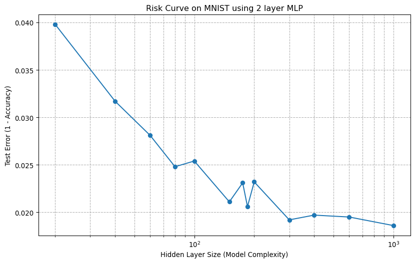
Double Descent Curve

# A wide range of hidden layer sizes to see the full curve
hidden_sizes = [20, 40, 60, 80, 100, 150, 175, 185, 200, 300, 400, 600, 1000]
test_errors = []

for size in hidden_sizes:
    print(f"Training a two-layer network with hidden layer size: {size}")

    # Create a two-layer network
    model = Sequential([
        Dense(size, activation="relu"),
        Dense(size, activation="relu"),
        Dense(10, activation="softmax")
    ])

    model.compile(
        optimizer="adam",
        loss="categorical_crossentropy",
        metrics=["accuracy"]
    )

    model.fit(x_train_flat, y_train, epochs=20, batch_size=128, verbose=0,
              validation_split=0.2)

    # Evaluate and store the test error (1 - accuracy)
    loss, accuracy = model.evaluate(x_test_flat, y_test, verbose=0)
    test_errors.append(1 - accuracy)

Training a two-layer network with hidden layer size: 20
Training a two-layer network with hidden layer size: 40
Training a two-layer network with hidden layer size: 60
Training a two-layer network with hidden layer size: 80
Training a two-layer network with hidden layer size: 100
Training a two-layer network with hidden layer size: 150
Training a two-layer network with hidden layer size: 175
Training a two-layer network with hidden layer size: 185
Training a two-layer network with hidden layer size: 200
Training a two-layer network with hidden layer size: 300
Training a two-layer network with hidden layer size: 400
Training a two-layer network with hidden layer size: 600
Training a two-layer network with hidden layer size: 1000

# Plotting the result
plt.figure(figsize=(10, 6))
plt.plot(hidden_sizes, test_errors, marker="o", linestyle="-")
plt.xscale("log")
plt.title("Risk Curve on MNIST using 2 layer MLP")
plt.xlabel("Hidden Layer Size (Model Complexity)")
plt.ylabel("Test Error (1 - Accuracy)")
plt.grid(True, which="both", ls="--")
plt.show()