description = 'Darrin William Stephens, SIT741: Statistical Data Analysis, Task T06.P6'Generalised Additive Models
Introduction
In this task, generalised additive model’s are explored for two datasets.
1. Define a string and print it
This section defines a string containing my name, the unit name and the task name.
Print the string using the cat() function.
cat(description)Darrin William Stephens, SIT741: Statistical Data Analysis, Task T06.P62. Read the first dataset
This part of the task uses the Afghanistan data from the gapminder dataset.
afghan_data = gapminder |>
  filter(country == "Afghanistan")
Fit a generalised additive model
Fitting generalised additive model that predicts life expectancy from the population using the default smoothing function. The histogram of life expectancy is shown below, it appears to resemble a normal distribution, although more more data would help.
afghan_data |>
  ggplot(aes(x=lifeExp)) +
  geom_histogram(bins=6, color="darkgray") +
  labs(title="Distribution of life expectancy", x="Life expectancy (years)", y="Count") +
  theme(plot.title=element_text(hjust=0.5))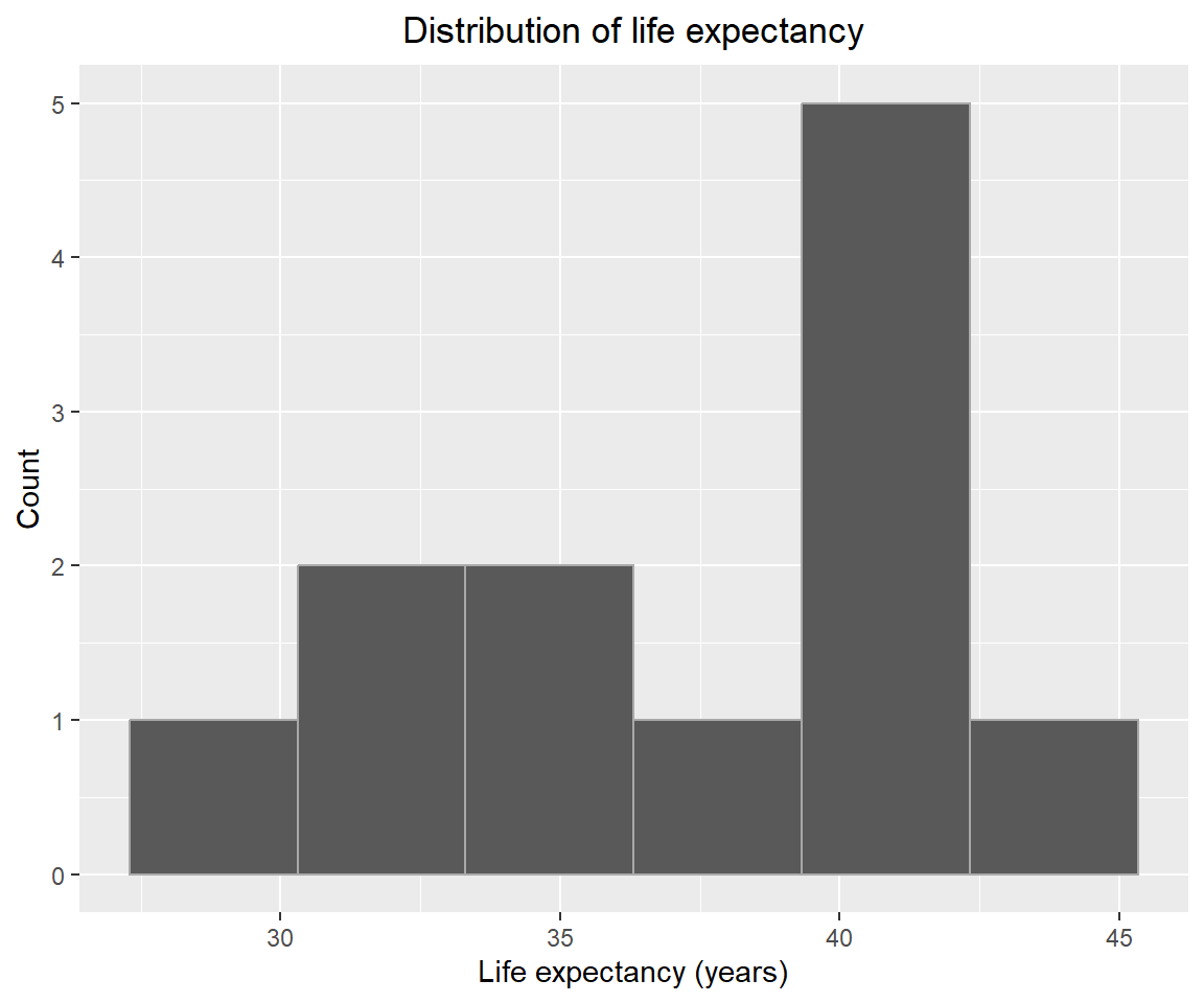
I have used a Gaussian distribution for the family based on the distribution of life expectancy.
gam_model = gam(lifeExp ~ s(pop), family=gaussian(link = "identity"), data = afghan_data)Model outputs
summary(gam_model)
Family: gaussian
Link function: identity

Formula:
lifeExp ~ s(pop)

Parametric coefficients:
            Estimate Std. Error t value Pr(>|t|)
(Intercept)  37.4788     0.4396   85.25 5.77e-13 ***
---
Signif. codes:  0 '***' 0.001 '**' 0.01 '*' 0.05 '.' 0.1 ' ' 1

Approximate significance of smooth terms:
         edf Ref.df     F p-value
s(pop) 3.123  3.754 29.85 7.7e-05 ***
---
Signif. codes:  0 '***' 0.001 '**' 0.01 '*' 0.05 '.' 0.1 ' ' 1

R-sq.(adj) =  0.911   Deviance explained = 93.6%
GCV = 3.5332  Scale est. = 2.3191    n = 12
The baseline life expectancy (intercept) is ~37.5 years and is highly significant. The estimated degrees of freedom for the smoothing is 3.1 suggesting it is non-linear. The p-value indicates the s(pop) is statistically significant, suggesting the population has a non-linear and meaningful effect on life expectancy.
plot(gam_model, shade = TRUE, main = "Effect of Population on Life Expectancy in Afghanistan")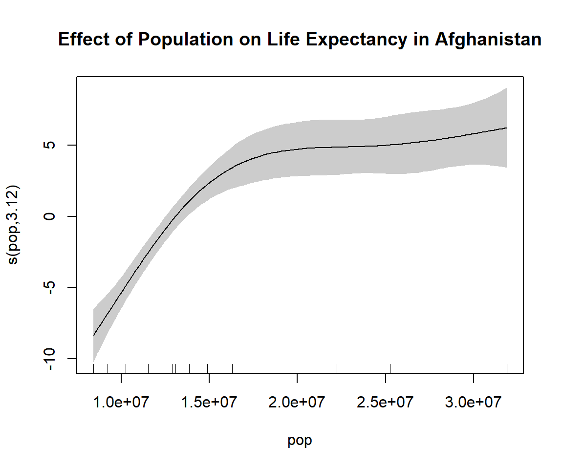
3. Re-fit with different smoother
The default smoother in gam(), is the thin plate regression splines. Here, I fit a new model using cubic regression splines for the smoothing function.
gam_model2_k10 = gam(lifeExp ~ s(pop, bs = "cr"),
                     family=gaussian(link = "identity"), data = afghan_data)
summary(gam_model2_k10)
Family: gaussian
Link function: identity

Formula:
lifeExp ~ s(pop, bs = "cr")

Parametric coefficients:
            Estimate Std. Error t value Pr(>|t|)
(Intercept)  37.4788     0.4374   85.69 5.16e-13 ***
---
Signif. codes:  0 '***' 0.001 '**' 0.01 '*' 0.05 '.' 0.1 ' ' 1

Approximate significance of smooth terms:
         edf Ref.df     F  p-value
s(pop) 3.099  3.686 30.73 7.01e-05 ***
---
Signif. codes:  0 '***' 0.001 '**' 0.01 '*' 0.05 '.' 0.1 ' ' 1

R-sq.(adj) =  0.912   Deviance explained = 93.7%
GCV = 3.4865  Scale est. = 2.2955    n = 12
Effect of k
The default k value for cubic regression splines is 10. Now, I’ll fit models with different values of k (3, 5, 7 and 10).
# Fit models with different k values
gam_model2_k3 = gam(lifeExp ~ s(pop, bs = "cr", k = 3),
                    family=gaussian(link = "identity"), data = afghan_data)
gam_model2_k5 = gam(lifeExp ~ s(pop, bs = "cr", k = 5),
                    family=gaussian(link = "identity"), data = afghan_data)
gam_model2_k7 = gam(lifeExp ~ s(pop, bs = "cr", k = 7),
                    family=gaussian(link = "identity"), data = afghan_data)

# Compare summaries
summary(gam_model2_k3)
Family: gaussian
Link function: identity

Formula:
lifeExp ~ s(pop, bs = "cr", k = 3)

Parametric coefficients:
            Estimate Std. Error t value Pr(>|t|)
(Intercept)   37.479      0.519   72.21 8.37e-14 ***
---
Signif. codes:  0 '***' 0.001 '**' 0.01 '*' 0.05 '.' 0.1 ' ' 1

Approximate significance of smooth terms:
         edf Ref.df     F  p-value
s(pop) 1.955  1.998 40.37 3.35e-05 ***
---
Signif. codes:  0 '***' 0.001 '**' 0.01 '*' 0.05 '.' 0.1 ' ' 1

R-sq.(adj) =  0.876   Deviance explained = 89.8%
GCV = 4.2883 Scale est. = 3.2324 n = 12summary(gam_model2_k5)
Family: gaussian
Link function: identity

Formula:
lifeExp ~ s(pop, bs = "cr", k = 5)

Parametric coefficients:
            Estimate Std. Error t value Pr(>|t|)
(Intercept)  37.4788     0.4239   88.42 3.37e-13 ***
---
Signif. codes:  0 '***' 0.001 '**' 0.01 '*' 0.05 '.' 0.1 ' ' 1

Approximate significance of smooth terms:
        edf Ref.df     F  p-value
s(pop) 3.04  3.408 36.14 4.17e-05 ***
---
Signif. codes:  0 '***' 0.001 '**' 0.01 '*' 0.05 '.' 0.1 ' ' 1

R-sq.(adj) =  0.917   Deviance explained =   94%
GCV = 3.2505 Scale est. = 2.1562 n = 12summary(gam_model2_k7)
Family: gaussian
Link function: identity

Formula:
lifeExp ~ s(pop, bs = "cr", k = 7)

Parametric coefficients:
            Estimate Std. Error t value Pr(>|t|)
(Intercept)  37.4788     0.4315   86.85 4.22e-13 ***
---
Signif. codes:  0 '***' 0.001 '**' 0.01 '*' 0.05 '.' 0.1 ' ' 1

Approximate significance of smooth terms:
         edf Ref.df     F  p-value
s(pop) 3.068  3.567 32.79 5.69e-05 ***
---
Signif. codes:  0 '***' 0.001 '**' 0.01 '*' 0.05 '.' 0.1 ' ' 1

R-sq.(adj) =  0.914   Deviance explained = 93.8%
GCV = 3.3806 Scale est. = 2.2346 n = 12summary(gam_model2_k10)
Family: gaussian
Link function: identity

Formula:
lifeExp ~ s(pop, bs = "cr")

Parametric coefficients:
            Estimate Std. Error t value Pr(>|t|)
(Intercept)  37.4788     0.4374   85.69 5.16e-13 ***
---
Signif. codes:  0 '***' 0.001 '**' 0.01 '*' 0.05 '.' 0.1 ' ' 1

Approximate significance of smooth terms:
         edf Ref.df     F  p-value
s(pop) 3.099  3.686 30.73 7.01e-05 ***
---
Signif. codes:  0 '***' 0.001 '**' 0.01 '*' 0.05 '.' 0.1 ' ' 1

R-sq.(adj) =  0.912   Deviance explained = 93.7%
GCV = 3.4865  Scale est. = 2.2955    n = 12
# Compare AIC values
AIC(gam_model2_k3, gam_model2_k5, gam_model2_k7, gam_model2_k10) df AIC
gam_model2_k3 3.954727 52.65060
gam_model2_k5 5.040060 48.42880
gam_model2_k7 5.068026 48.87126
gam_model2_k10 5.099353 49.20891As k is increased from 3 to 10 the Deviance explained increase then decreases and the AIC value decreases then increases. From the k values tested, k=5 gives the highest Deviance explained and the lowest AIC value.
par(mfrow = c(2, 2))
plot(gam_model2_k3, shade = TRUE, main = "Cubic Regression Spline (k=3)")
plot(gam_model2_k5, shade = TRUE, main = "Cubic Regression Spline (k=5)")
plot(gam_model2_k7, shade = TRUE, main = "Cubic Regression Spline (k=7)")
plot(gam_model2_k10, shade = TRUE, main = "Cubic Regression Spline (k=10)")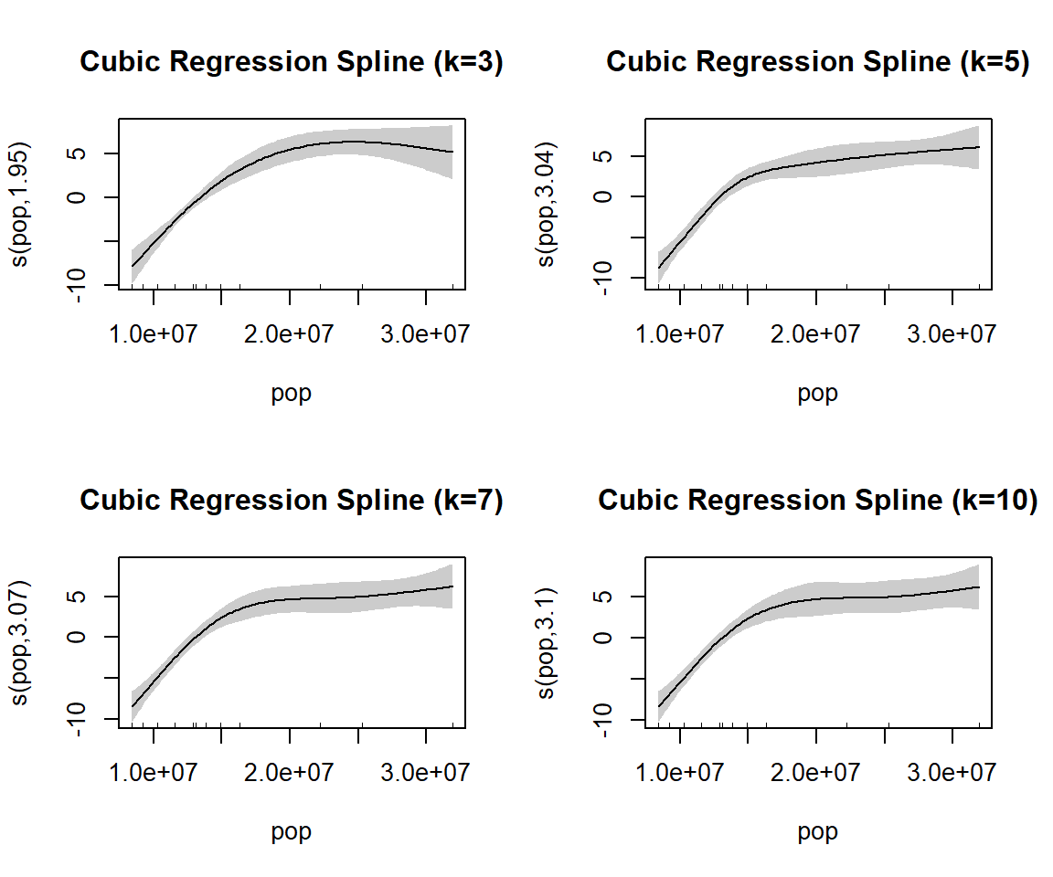
4. Read the second dataset
This section uses a dataset on abalone from https://archive.ics.uci.edu/dataset/1/abalone. The data is read and columns renamed to have appropriate labels. then convert the “rings” into the “age” as suggested by the dataset source.
abalone = read.table(
  "http://archive.ics.uci.edu/ml/machine-learning-databases/abalone/abalone.data", sep = ",")

# Rename columns
abalone_df = abalone |>
  rename(
    sex=V1,
    length=V2,
    diameter=V3,
    height=V4,
    whole_weight=V5,
    shucked_weight=V6,
    viscera_weight=V7,
    shell_weight=V8,
    rings=V9
  )

glimpse(abalone_df)
Rows: 4,177
Columns: 9
$ sex <chr> "M", "M", "F", "M", "I", "I", "F", "F", "M", "F", "F", …
$ length <dbl> 0.455, 0.350, 0.530, 0.440, 0.330, 0.425, 0.530, 0.545,…
$ diameter <dbl> 0.365, 0.265, 0.420, 0.365, 0.255, 0.300, 0.415, 0.425,…
$ height <dbl> 0.095, 0.090, 0.135, 0.125, 0.080, 0.095, 0.150, 0.125,…
$ whole_weight <dbl> 0.5140, 0.2255, 0.6770, 0.5160, 0.2050, 0.3515, 0.7775,…
$ shucked_weight <dbl> 0.2245, 0.0995, 0.2565, 0.2155, 0.0895, 0.1410, 0.2370,…
$ viscera_weight <dbl> 0.1010, 0.0485, 0.1415, 0.1140, 0.0395, 0.0775, 0.1415,…
$ shell_weight <dbl> 0.150, 0.070, 0.210, 0.155, 0.055, 0.120, 0.330, 0.260,…
$ rings <int> 15, 7, 9, 10, 7, 8, 20, 16, 9, 19, 14, 10, 11, 10, 10, …# Convert "rings" to "age" by adding 1.5 (as per dataset documentation)
abalone_df = abalone_df |>
mutate(
age=rings + 1.5,
)Create training/test sets
Create training and test sets using a 10-fold cross-validation.
# Create 10-fold cross-validation splits
set.seed(42)
cv_splits = vfold_cv(abalone_df, v = 10)

for (i in seq_along(cv_splits$splits)) {
  cat("Fold", i, "\n")

  print(cv_splits$splits[[i]])
  cat("\n")
}
Fold 1
<Analysis/Assess/Total>
<3759/418/4177>
Fold 2
<Analysis/Assess/Total>
<3759/418/4177>
Fold 3
<Analysis/Assess/Total>
<3759/418/4177>
Fold 4
<Analysis/Assess/Total>
<3759/418/4177>
Fold 5
<Analysis/Assess/Total>
<3759/418/4177>
Fold 6
<Analysis/Assess/Total>
<3759/418/4177>
Fold 7
<Analysis/Assess/Total>
<3759/418/4177>
Fold 8
<Analysis/Assess/Total>
<3760/417/4177>
Fold 9
<Analysis/Assess/Total>
<3760/417/4177>
Fold 10
<Analysis/Assess/Total>
<3760/417/4177>5. Fit a generalised additive model
In this section I look at fitting a model that predicts the age of abalone from Shell Weight, Diameter and Length.
The fit_gam and predict_gam function have been copied from the Week 10 R activity.
fit_gam <- function(splt, ...)
  gam(..., data = analysis(splt))

predict_gam <- function(splt, mod, ...)
  broom::augment(mod, newdata = assessment(splt))
In a previous task it was shown that the distribution of Age looks normal with some positive skew. I will use Gaussian for the family and “identity” for the link function.
cv_splits = cv_splits |>
  mutate(models = map(splits,
                      fit_gam,
                      age ~ s(shell_weight) + s(diameter) + s(length),
                      )
         )
We can generate predictions for each fold using the predict_gam function..
cv_splits <- cv_splits |>
  mutate(predictions = map2(splits,
                            models,
                            predict_gam)
         )

cv_splits
# 10-fold cross-validation
# A tibble: 10 × 4
splits id models predictions
<list> <chr> <list> <list>
1 <split [3759/418]> Fold01 <gam> <tibble [418 × 12]>
2 <split [3759/418]> Fold02 <gam> <tibble [418 × 12]>
3 <split [3759/418]> Fold03 <gam> <tibble [418 × 12]>
4 <split [3759/418]> Fold04 <gam> <tibble [418 × 12]>
5 <split [3759/418]> Fold05 <gam> <tibble [418 × 12]>
6 <split [3759/418]> Fold06 <gam> <tibble [418 × 12]>
7 <split [3759/418]> Fold07 <gam> <tibble [418 × 12]>
8 <split [3760/417]> Fold08 <gam> <tibble [417 × 12]>
9 <split [3760/417]> Fold09 <gam> <tibble [417 × 12]>
10 <split [3760/417]> Fold10 <gam> <tibble [417 × 12]>6. Erorrs and variation in cross-validation
Then we can calculate the error of each fold. Here I have used the RMSE and MAE error metrics.
library(yardstick)
cv_splits <- cv_splits |>
  mutate(
    rmse = map_dbl(predictions, function(x, ...) rmse(x, ...)$.estimate, age, .fitted),
    mae  = map_dbl(predictions, function(x, ...) mae(x, ...)$.estimate,  age, .fitted)
  )

cv_splits
# 10-fold cross-validation
# A tibble: 10 × 6
splits id models predictions rmse mae
<list> <chr> <list> <list> <dbl> <dbl>
1 <split [3759/418]> Fold01 <gam> <tibble [418 × 12]> 2.36 1.73
2 <split [3759/418]> Fold02 <gam> <tibble [418 × 12]> 2.19 1.62
3 <split [3759/418]> Fold03 <gam> <tibble [418 × 12]> 2.28 1.65
4 <split [3759/418]> Fold04 <gam> <tibble [418 × 12]> 2.22 1.61
5 <split [3759/418]> Fold05 <gam> <tibble [418 × 12]> 2.44 1.70
6 <split [3759/418]> Fold06 <gam> <tibble [418 × 12]> 2.33 1.70
7 <split [3759/418]> Fold07 <gam> <tibble [418 × 12]> 2.30 1.56
8 <split [3760/417]> Fold08 <gam> <tibble [417 × 12]> 2.24 1.63
9 <split [3760/417]> Fold09 <gam> <tibble [417 × 12]> 2.40 1.73
10 <split [3760/417]> Fold10 <gam> <tibble [417 × 12]> 2.46 1.75# Create a dataframe with the error for each fold
error_df <- cv_splits |>
select(rmse, mae) |>
mutate(fold = row_number()) |>
pivot_longer(cols = c(rmse, mae), names_to = "metric", values_to = "value")
# Calculate summary statistics
summary_stats <- error_df |>
group_by(metric) |>
summarise(mean = mean(value), sd = sd(value), .groups = "drop")
# Plot
ggplot(error_df, aes(x = fold, y = value, color = metric)) +
geom_line() +
geom_point(size = 2) +
geom_hline(data = summary_stats, aes(yintercept = mean, color = metric),
linetype = "dashed", show.legend = FALSE) +
labs(
title = "Error Variation Across CV Folds with Mean",
x = "Fold",
y = "Error",
color = "Metric"
) +
theme(plot.title=element_text(hjust=0.5))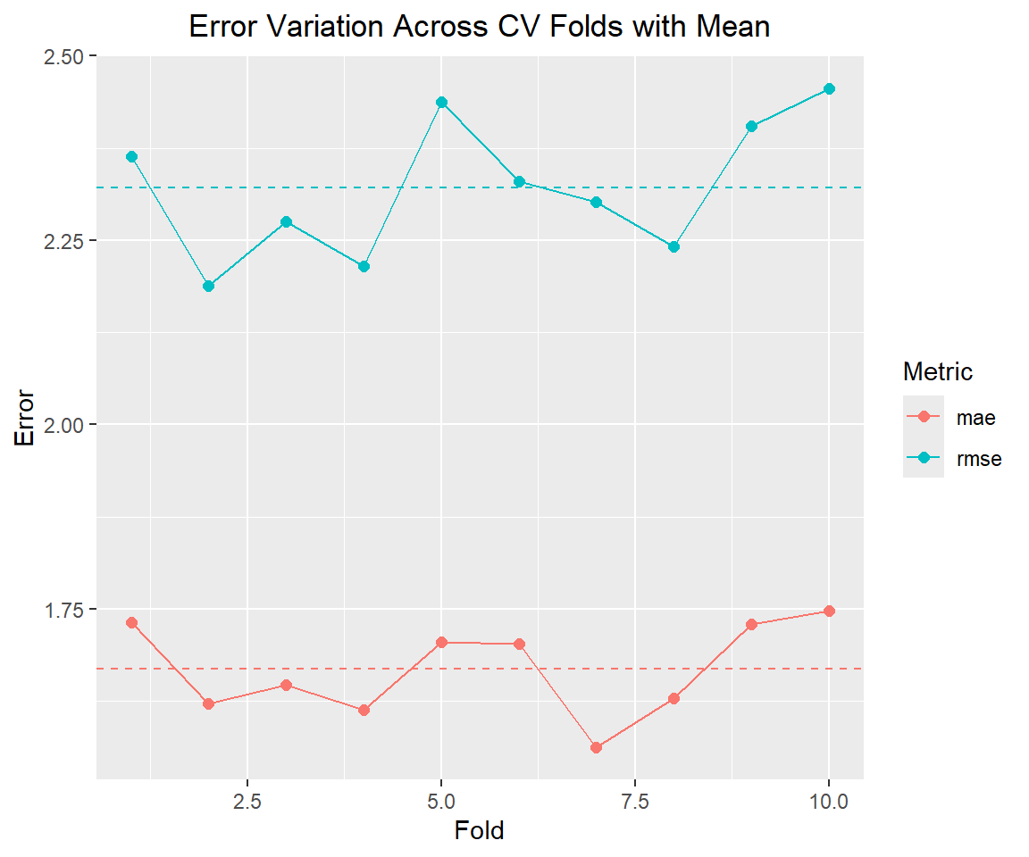
# Summary of variation
print(summary_stats)
# A tibble: 2 × 3
metric mean sd
<chr> <dbl> <dbl>
1 mae 1.67 0.0625
2 rmse 2.32 0.0934